LEJPT - Leonardo Electronic Journal of Practices and Technologies

Warning: include(/home/www/data/lejpthead.php): failed to open stream: No such file or directory in /home/www/data/lejpt/gettext.php on line 4

Warning: include(): Failed opening '/home/www/data/lejpthead.php' for inclusion (include_path='.:/usr/pkg/lib/php') in /home/www/data/lejpt/gettext.php on line 4
LEJPT - Leonardo Electronic Journal of Practices and Technologies - light html archive A01
Warning: include(/home/www/data/lejptbody.php): failed to open stream: No such file or directory in /home/www/data/lejpt/gettext.php on line 6

Warning: include(): Failed opening '/home/www/data/lejptbody.php' for inclusion (include_path='.:/usr/pkg/lib/php') in /home/www/data/lejpt/gettext.php on line 6
Leonardo Electronic Journal of Practices and Technologies

Issue 01, p. 01-18
Topological Substituent Descriptors
Mircea V. DIUDEA^1*, Lorentz JÄNTSCHI², Ljupčo PEJOV³
¹"Babeş-Bolyai" University Cluj-Napoca, Romania
²Technical University Cluj-Napoca, Romania
³"Sv. Kiril i Metodij" University Skopje, Macedonia
*corresponding author, diudea@chem.ubbcluj.ro

Abstract
Motivation. Substituted 1,3,5-triazines are known as useful herbicidal substances. In view of reducing the cost of biological screening, computational methods are carried out for evaluating the biological activity of organic compounds. Often a class of bioactives differs only in the substituent attached to a basic skeleton. In such cases substituent descriptors will give the same prospecting results as in case of using the whole molecule description, but with significantly reduced computational time. Such descriptors are useful in describing steric effects involved in chemical reactions.
Method. Molecular topology is the method used for substituent description and multi linear regression analysis as a statistical tool.
Results. Novel topological descriptors, X_LDS and W_s, based on the layer matrix of distance sums and walks in molecular graphs, respectively, are proposed for describing the topology of substituents linked on a chemical skeleton. They are tested for modeling the esterification reaction in the class of benzoic acids and herbicidal activity of 2-difluoromethylthio-4,6-bis(monoalkylamino)-1,3,5-triazines.
Conclusions. Ws substituent descriptor, based on walks in graph, satisfactorily describes the steric effect of alkyl substituents behaving in esterification reaction, with good correlations to the Taft and Charton steric parameters, respectively. Modeling the herbicidal activity of the seo of 1,3,5-triazines exceeded the models reported in literature, so far.
Keywords
Steric effect, Substituent descriptors, Molecular topology, Herbicidal activity. Abbreviations and notations MLR, multi linear regression; SVTI, substituent volume topological index; E_s, Taft’s steric parameter; n, Charton’s steric parameter.

1. Introduction
In the field of chemical reactivity, the first proposal of a substituent steric parameter is due to Taft [1, 2]. He tried to quantify the steric influence of a substituent located on the hydrocarbon part of organic esters in the acid-catalysed hydrolysis of aliphatic carboxylic esters, RCOOR’. His E_s steric parameter is defined as:
(1)
where is the ratio of acid-catalysed hydrolysis rate constant of RCOOR’ to that of MeCOOR’. By definition, .
The E_s parameter has been defined empirically [3]. Taft himself pointed out that E_s varies parallel to the atom group radius. Charton also found that E_s is linearly dependent on the van der Waals radius of the substituent, thus defining a new steric parameter, n [4-8]. Murray [9] found correlations between the Taft parameter and the Randić [10] topological index, for a series of substituted alkyls. In this respect, Ivanciuc and Balaban [3] have proposed a topological descriptor, SVTI, which encodes the topological distances (i.e., the number of bonds/edges, D_ij, joining the atoms/vertices i and j on the shortest path) in a molecular graph, G. It is defined on the fragment F (i.e. an alkyl group) attached to the vertex i of G, as:
(2)
The summation runs over all N_F vertices of F and the distance D_ijis limited to 3, in agreement to the Charton’s conclusion about the limit of the influence of the steric effect beyond the gamma carbon [5-8]. The calculation of SVTI is exemplified for the sec-butyl group (R = H) or higher homologues (R ¹ H):

SVTI (s-Bu) = 1+ 2 + 2 + 3 = 8
The above authors have tested their descriptors in describing the reaction rates of acid-catalysed hydrolysis of RCOOR' (the Taft's set). In the present work, two novel descriptors for substituents are proposed. They are now tested in modeling the effector-receptor interaction in the herbicidal activity of 2-difluoromethylthio-4,6-bis(monoalkylamino)-1,3,5-triazines.

2. Substituent Topological Descriptors, X_LDSand W_s
The substituent descriptors X_LDS and W_s herein proposed are constructed with the aid of layer matrices. Before defining our descriptors, let’s recall some knowledges about the layer matrices [11-17]. A partition G(i) with respect to the vertex i, in a graph, is defined [11, 14, 15] as:
(3)
where D_iu is the topological distance (see above) and ecc_i is the eccentricity of i (i.e. the largest distance between i and any vertex in G). Figure 1 illustrates the relative partitions for the graph G₁. Let be the layer j of the vertices u located at distance j, in the relative partition G(i): (4) The entries in a layer matrix, LM, collect the topological property P_u for all vertices u belonging to the layer :
(5)


G₁	G₁(1,5)	G₁(2)	G₁(3)	G₁(4)

G₁(1) = {{1},{2},{3,5},{4}}; G₁(2) = {{2},{1,3,5},{4}}; G₁(3) = {{3},{2,4},{1,5}}; G₁(4) = {{4},{3},{2},{1,5}}; G₁(5) = {{5},{2},{1,3},{4}}. Figure 1. Partitions of G₁with respect to each of its vertices
The matrix LM can be written as:
(6) LM(G)=
where V(G) is the set of vertices in graph and d(G) is the diameter (i.e., the largest distance) of G. The dimensions of such a matrix are N´ (d(G)+1). Figure 2 illustrates the layer matrix of distance sums, LDS [13], the topological property M which collects being the sum of distances joining a vertex i with all the remainder vertices in G. Note that the first column contains just the vertex topological property. (in this case, , marked in the weighted graph, G₂{DS_i}).

G₂

i\j:	0	1	2	3	4
(1)	15	10	24	26	17
(2)	10	39	26	17	0
(3)	9	36	47	0	0
(4)	12	26	24	30	0
(5)	17	12	9	24	30
(6)	15	10	24	26	17
(7)	14	9	22	47	0

LDS(G₂)

Figure 2. Matrix LDS for the graph G₂
This matrix and the invariants calculated on (e.g., the well-known Wiener index [18], counting all distances in G) are useful tools in topological description of molecular graphs [13, 14]. Another interesting matrix is the layer matrix of walk degrees [15], L^eW. A walk, W, is defined [19] as a continuous sequence of vertices, v₁, v₂, ..., v_m; it is allowed edges and vertices to be revisited. If the two terminal vertices coincide (v₁= v_m ), the walk is called a closed (or self returning) walk, otherwise it is an open walk. If its vertices are distinct, the walk is called a path. The number e of edges traversed is called the length of walk. Walks of length e, starting at the vertex i, ^eW(i), can be counted by summing the entries in the row i of the e^th power of the adjacency matrix A (whose nondiagonal entries are 1 if two atoms are adjacent and zero otherwise):
(7)
where ^eW(i) is called the walk degree (of rank e) of vertex i (or atomic walk count [15, 20] ). Walk degrees, ^eW(i), can be also calculated by summing the first neighbours degrees of lower rank, according to an additive algorithm¹¹ illustrated in figures 3 and 4. Local and global invariants based on walks in graph were considered for correlating with physico-chemical properties [15, 20]. Figure 3 illustrates the layer matrix of walk degrees, L^eW, e = 1-4, for G₂. Note that the first column in L¹W is just the vertex degree or the vertex valency. Note that the matrix L^eW was re-invented by Randic in 2001, for e = 1, under the name "valence shells" [21]. The substituent descriptor X_LDS is the local "centrocomplexity index", X_LM [14], defined on the LDS matrix:
(8)
where i is the attachment point of the substituent to a given chemical structure (see figure 4) and z denotes the number of bits of max[LDS]_ij in G. Calculation of X_LDS is exemplified in figure 4.


	G₂ {¹W_i}	G₂ {²W_i}	G₂ {³W_i}	G₂ {⁴W_i}
	L¹W	L²W	L³W	L⁴W
i\j	0 1 2 3 4	0 1 2 3 4	0 1 2 3 4	0 1 2 3 4
1	1 3 4 3 1	3 5 9 7 2	5 12 17 14 4	12 22 38 28 8
2	3 5 3 1 0	5 12 7 2 0	12 22 14 4 0	22 50 28 8 0
3	3 6 3 0 0	6 12 8 0 0	12 26 14 0 0	26 50 32 0 0
4	2 4 4 2 0	4 8 8 6 2	8 16 18 10 0	16 34 34 24 0
5	1 2 3 4 2	2 4 6 8 6	4 8 12 18 10	8 16 26 34 24
6	1 3 4 3 1	3 5 9 7 2	5 12 17 14 4	12 22 38 28 8
7	1 3 5 3 0	3 6 9 8 0	6 12 20 14 0	12 26 38 32 0

Figure 3. Layer matrix of walk degrees, L^eW for the graph G₂ (calculated by summing the first neighbor degrees of lower rank)


{¹W}	{²W}	{³W}	{DS}	(a)
W_s (i) = 7+7/2+11/3+8/4 ≈ 16.167; X_LDS(i) = 14∙10⁰+10∙10^-2+8∙10^-4+8∙10^-6+12∙10^-8+12∙10^-10 = 14.1008081212 ≈ 14.101;				(b)

Figure 4. (a) Walk degrees, ^eW, (calculated by summing the first neighbors degrees of lower rank) and distance sums, DS; (b) Evaluation of W_s and X_LDS descriptors
W_sis based on the walks in a connected molecular graph. It is calculated from the layer matrix L³W by:
(9)
where ³W is the walk number, of length 3. We limited here to elongation 3 by following the Charton’s suggestion about the limit of the influence of steric effect (see above). The calculation of the parameter W_s is exemplified in figure 4. The X_LDS descriptor is similar to the SVTI parameter, both of them counting distances in the substituent. W_s describes the branching in the vicinity of the attachment point i. All these parameters suggest the steric influence of a substituent in the interaction of the skeleton (or a situs of it) with a partner (e.g., a reactant [3, 22] or a biological receptor). They are free of electronic contributions, at least in the variant in which the heteroatom is not considered.

3. Correlating Test
The utility of the substituent descriptors, X_LDS and W_s, was proven on a set of thirty aminoalkyl fragments (table 1) involved in the inhibition of Hill reaction of triazines [23] (figure 5). In this respect, the fragmental volumes, V, (in cm³/mol) for the considered substituents have been calculated as described below. Other parameter herein considered was the number of atoms different from hydrogen, N. All these descriptors have been calculated separately for the two sites, A and B (see figure 5).

Figure 5. Herbicidal bioactive triazines
Table 1. Topological descriptors and biological activity pI₅₀ for the triazines in figure 5

No	A	B	N_A	N_B	W_s,_A	W_s,_B	X_A^*	X_B	V_A^**	V_B	pI₅₀
1	NH₂	NH₂	1	1	1	1	1.1	1.1	18.763	18.763	3.82
2	NH₂	NHCH₃	1	2	1	5	1.1	3.23	18.763	32.636	5.20
3	NH₂	NHC₂H₅	1	3	1	8.5	1.1	6.446	18.763	47.908	5.34
4	NH₂	NH-i-C₃H₇	1	4	1	13.66	1.1	9.061	18.763	60.766	5.83
5	NHCH₃	NHCH₃	2	2	5	5	3.23	3.23	32.636	32.636	6.01
6	NHCH₃	NHC₂H₅	2	3	5	8.5	3.23	6.446	32.636	47.908	6.39
7	NHCH₃	NHC₃H₇	2	4	5	11.75	3.23	10.071	32.636	62.393	6.75
8	NHCH₃	NH-i-C₃H₇	2	4	5	13.66	3.23	9.061	32.636	60.766	6.76
9	NHCH₃	NHC₄H₉	2	5	5	13.93	3.23	15.111	32.636	76.638	6.74
10	NHCH₃	NH-s-C₄H₉	2	5	5	15.16	3.23	13.091	32.636	75.039	6.76
11	NHCH₃	NH-t-C₄H₉	2	5	5	20.50	3.23	12.081	32.636	74.106	6.78
12	NHCH₃	NHC₅H₁₁	2	6	5	15.62	3.23	21.161	32.636	88.241	7.12
13	NHC₂H₅	NHC₂H₅	3	3	8.5	8.5	6.446	6.446	47.908	47.908	6.82
14	NHC₂H₅	NHC₃H₇	3	4	8.5	11.75	6.446	10.071	47.908	62.393	6.74
15	NHC₂H₅	NH-i-C₃H₇	3	4	8.5	13.66	6.446	9.061	47.908	60.766	6.89
16	NHC₂H₅	NHC₄H₉	3	5	8.5	13.93	6.446	15.111	47.908	76.638	6.95
17	NHC₂H₅	NH-i-C₄H₉	3	5	8.5	16.16	6.446	14.101	47.908	74.497	7.01
18	NHC₂H₅	NH-s-C₄H₉	3	5	8.5	15.16	6.446	13.091	47.908	75.039	6.87
19	NHC₂H₅	NH-t-C₄H₉	3	5	8.5	20.50	6.446	12.081	47.908	74.106	6.97
20	NHC₂H₅	NHC₅H₁₁	3	6	8.5	15.62	6.446	21.161	47.908	88.241	6.94
21	NHC₂H₅	NHC₆H₁₃	3	7	8.5	17.00	6.446	28.222	47.908	102.032	7.21
22	NHC₂H₅	NHC₇H₁₅	3	8	8.5	18.17	6.446	36.292	47.908	116.672	7.01
23	NHC₂H₅	NHC₈H₁₇	3	9	8.5	19.18	6.446	45.373	47.908	128.770	6.81
24	NHC₃H₇	NHC₃H₇	4	4	11.75	11.75	10.071	10.071	62.393	62.393	6.45
25	NH-i-C₃H₇	NHC₃H₇	4	4	13.66	11.75	9.061	10.071	60.766	62.393	6.75
26	NH-i-C₃H₇	NH-i-C₃H₇	4	4	13.66	13.66	9.061	9.061	60.766	60.766	6.75
27	NH-i-C₃H₇	NHC₄H₉	4	5	13.66	13.93	9.061	15.111	60.766	76.638	6.71
28	NH-i-C₃H₇	NH-s-C₄H₉	4	5	13.66	15.16	9.061	13.091	60.766	75.039	6.88
29	NH-i-C₃H₇	NH-t-C₄H₉	4	5	13.66	20.50	9.061	12.081	60.766	74.106	6.70
30	NH-i-C₃H₇	NHC₅H₁₁	4	6	13.66	15.62	9.061	21.161	60.766	88.241	6.69

* The symbol X stands for X_LDS (see text);
** Volume, [cm³/mol].
Table 2. Statistics of multivariable regression (distinct variables on branches A and B)

No.	X_I	b_i	A	r	s	v(%)	F
1	1/N,_B	-3.786	7.549	0.8987	0.311	4.752	117.587
2	1/W_s_,B	-3.372	6.933	0.8298	0.396	6.047	61.899
3	1/X_B	-3.806	7.038	0.8835	0.333	5.076	99.598
4	1/V_B	-72.276	7.760	0.8975	0.313	4.779	115.936
5	1/N_A1/N_B	-1.234-2.678	7.810	0.9577	0.208	3.175	149.557
6	1/W_s,_A1/W_s,_B	-1.335-2.077	7.118	0.9615	0.199	3.030	165.554
7	1/X_A1/X_B	-1.317-2.526	7.252	0.9662	0.186	2.844	189.755
8	1/V_A1/V_B	-22.999-52.514	8.048	0.9478	0.231	3.519	119.237
9	1/W_s,_A1/V_B	-1.114-47.194	7.618	0.9714	0.172	2.619	226.162
10	1/W_s,_A1/X_B	-1.180-2.458	7.159	0.9729	0.167	2.550	239.280
11	1/W_s,_A1/N_B	-1.120-2.484	7.484	0.9746	0.162	2.472	255.491
12	N_A1/N_A1/N_B	-0.385-2.777-2.444	9.477	0.9834	0.134	2.039	254.937
13	W_s,_A1/W_s,_A1/W_s,_B	-0.025-1.594-2.056	7.372	0.9661	0.190	2.903	121.327
14	X_A1/X_A1/X_B	-0.078-2.047-2.413	7.876	0.9818	0.140	2.132	232.401
15	V_A1/V_A1/V_B	-0.036-65.998-45.367	10.649	0.9808	0.144	2.193	219.227
16	X_A1/V_A1/V_B	-0.155-59.011-46.244	9.762	0.9815	0.141	2.152	228.039
17	X_A1/V_A1/X_B	-0.154-60.818-2.399	9.337	0.9836	0.133	2.029	257.426
18	X_A1/V_A1/N_B	-0.153-58.888-2.430	9.614	0.9846	0.129	1.968	274.318

In table 2 A and b_i values are the coefficients of:
(10)
and leave one out procedure (loo) has the results:
(11) loo(12): r = 0.9768; s = 0.153; v(%) = 2.332; loo(18): r = 0.9778; s = 0.149; v(%) = 2.271.
The inhibitory activities of triazines on Chlorella have been taken from the study of Morita et al [24]. They are expressed as pI50, which represents the negative logarithm of concentration required for 50% inhibition of Hill reaction. The correlating results are listed in table 2. 4. Results and Discussion In single variable regression, the descriptors for the substituents in branch B (table 2) are not satisfactory to model the inhibitory activity of triazines; the correlation coefficient, r, is lower than 0.9 (for those in A, r is still lower) and the coefficient of variance, v, is about 5 %. Note that all these "steric" descriptors are taken as reciprocal values, suggesting that the triazine ring fits at the biological receptor as better as the substituent is less sterically involved. In two variables regression, by adding the descriptors for the branch A the correlation is improved, as indicates the higher values for r and F (the Fisher ratio) and the drop in the dispersion, s, and v(%) values (entries 5-8, table 2). When the descriptors for the two branches are heterogeneous, the result is still better (entries 9-11). In three variables regression, the correlation is once more improved. Again the heterogeneous descriptors model the inhibition reaction better that the homogeneous ones (compare entries 16-18 with 12-15, Table 2). The best model found (see also entry 18) was:
(12) pI₅₀ = 9.614 – 0.153∙X_A – 58.888∙1/V_A – 2.430∙1/N_B; n = 30; r² = 0.9694; s = 0.129; v(%) = 1.968; F = 274.3;
The cross validation (leave-one-out, "loo", procedure) test for the equations in entries 12 and 18 are given in the bottom of table 2. Despite the excellent model offered by equation (10), a brief inspection on the general structure of these triazines showed a rather surprising error: the molecule is symmetric, so that the two branches A and B are interchangeable! In consequence, the two columns of descriptors have no meaning if they are taken as distinct descriptors. Thus, the contribution of the substituents in A and B in modeling the global biological activity must somehow be mixed! The simple summation (or simple arithmetic mean) of contributions of the two branches, A and B, did not provide satisfactory results. More reliable appeared in other kinds of average: geometric ("geo") and harmonic ("har"). The best correlating results are included in table 3. The cross validation test, loo, is given for each entry. From table 3 it appears that, in single variable regression, the descriptor 1/X_(LDS)geo provides a rather good (r> 0.95) description of the activity, both in estimation and prediction, "loo" (entry 2). The best prediction is offered by the three variables equation, in entry 6 (r >0.975), all of them as harmonic average of the descriptors of A and B branches:
(13) pI₅₀ = 10.292 – 119.503∙1/V_har – 0.097∙X_har – 0.047∙W_s_,har; n = 30; r = 0.9807; s = 0.144; v(%) = 2.198; F = 218.158;
The corresponding arithmetic averaged descriptors used in (11) supplied a correlation of r = 0.955 which is, of course, unsatisfactory. This equation was chosen for a tempting prediction in the past. The experimental data for the compounds no. 3, 12, 21 and 24 (showing residuals, y_calc-y_exp, about two times or larger than the value of standard error of estimate: s = +0.144; -0.254; +0.236; +0.301 and -0.398, respectively were changed by the values: 5.6209; 6.8778; 6.9073 and 6.8471, respectively calculated by equations:
(14) pI₅₀ = 10.292 – 119.503 1/V_har – 0.097 X_har – 0.047 W_s_,har n = 26; r = 0.9932; s = 0.086; v(%) = 1.309; F = 530.484
The correlating data, obtained by using the new column of activities, y_cor, are included in table 3 as the rows "y_cor". The improvement in the statistical parameters of the regression equations is obvious for all data of table 3 (where ^* means "leave one out" cross validation procedure; and ^** are y_i corrected for i = 3, 12, 21 and 24):
Table 3. Statistics of multivariable regression, Y_calc = a + Σ_i b_iX_i (averaged variables)

No.	X_i	b_i	a	r	s	v(%)	F
1	1/W_s,harloo^y_cor^*	-3.151	7.121	0.9553 0.9467 0.9666	0.210 0.229 0.175	3.204 3.489 2.669	292.215 398.721
2	1/X_geolooy_cor	-3.891	7.253	0.9621 0.9558 0.9793	0.194 0.209 0.138	2.956 3.183 2.108	348.097 655.776
3	1/V_harN_harlooy_cor	-126.800 -0.541	11.091	0.9763 0.9721 0.9924	0.156 0.167 0.086	2.387 2.543 1.307	275.063 875.466
4	1/V_harX_harlooy_cor	-113.340 -0.137	10.010	0.9777 0.9735 0.9907	0.152 0.163 0.095	2.318 2.480 1.446	292.278 713.286
5	1/N_harX_harW_s,harlooy_cor	-5.614 -0.056 -0.057	9.491	0.9798 0.9742 0.9918	0.147 0.160 0.091	2.247 2.446 1.380	208.342 523.336
6	1/V_harX_harW_s,harlooy_cor	-119.503 -0.097 -0.047	10.292	0.9807 0.9752 0.9938	0.144 0.157 0.079	2.198 2.397 1.204	218.158 690.328
7	1/V_harX_harW_s,harN_harlooy_cor	-105.131 -0.232 -0.081 0.673	9.058	0.9824 0.9742 0.9938	0.141 0.160 0.080	2.144 2.444 1.226	172.608 499.253
8	1/N_harX_harW_s,harV_harlooy_cor	-4.724 -0.228 -0.070 0.052	7.858	0.9825 0.9751 0.9924	0.140 0.157 0.089	2.139 2.401 1.358	173.400 405.773

More over, among the 24 descriptors (N, V, W_s, X_LDS, 1/N, 1/V, 1/W_s, 1/X_LDS, taken as "ari", "har" and "geo" average) used in single variable regression, in 20 of them an improvement of the statistics was recorded. Again the equation in entry 6 was the best model. This test suggested that the experimental data for the compounds, above mentioned, are "in error". From eq 11 and table 3, it comes out that the inhibitory activity of triazines is controlled by the possibility of the triazine ring (i.e., the pharmacophor) to accommodate at the receptor situs. This opinion is supported by the reciprocal values and the negative regression coefficient, and negative partial correlation index of these "steric" descriptors involved in an eq. of type 11. It suggests that the triazine ring fits at the biological receptor as better as the substituent is less sterically involved. A plot of the observed vs. calculated (by eq 11) pI₅₀ values is given in figure 6. For comparison, the plot for the same descriptors and "y_cor" is given in Figure 7.

Figure 6. Plot of experimental biological activity (VAR1) vs. y_calc. (cf. eq 11) values

Figure 7. Plot of experimental biological activity (VAR1) vs. y_cor values

4. Computation of Fragmental Volumes
The geometries of the hydrocarbon fragments (in fact, the corresponding radicals) were fully optimized at the Unrestricted Hartree-Fock (UHF) level of theory, using the 6-31G** basis set (of DZP quality), which contains a single set of d polarization functions on carbons, and a single set of p polarization functions on hydrogens for better description of the radical wavefunctions. The Berny's optimization algorithm was used (the energy derivatives with respect to nuclear coordinates were computed analytically [25]), along with the initial guess of the second derivative matrix. Standard harmonic vibrational analysis was applied to test the character of the optimized geometries (stationary points at the potential energy hypersurfaces - PES). All stationary points corresponded to real minima on the explored PES. Molecular volume calculations were performed for the optimized structures, by the Monte-Carlo method. Since Monte-Carlo method for calculating molecular volume (defined as the volume inside a contour of 0.001 electrons/Bohr³ density) is stochastically based algorithm, it often leads to results accurate up to several percents. Therefore, 11 volume calculations per fragment were performed for each fragment, and the arithmetic average value was taken as the closest approximation to the real one (at the level of theory employed). In order to increase the density of points for a more accurate integration, the "Tight" option of the Gaussian "Volume" keyword was used. All calculations were performed with Gaussian 94 suite of programs [26].

5. Conclusions
The W_s descriptor, based on the walks in graph, satisfactorily describes the steric effect of alkyl substituents in the esterification reaction. It is a pure steric parameter, not affected by the electronic effects. W_s correlate well to the fragmental volumes (over 0.92) and show a lower degeneracy in comparison to the SVTI, n and N_c parameters. It is also well correlated [18] to the Taft, E_s, (0.9637), and Charton, n, (0.9587), parameters, which makes from W_s a promising alternative in describing the steric effect of alkyl substituents.

6. Acknowledgment
The work was supported in part by the Romanian GRANT CNCSIS 2002.

References
[1] R. W. Taft, Linear free energy relationships from rates of esterification and hydrolysis of aliphatic and ortho-substituted benzoate esters. J. Am. Chem. Soc. 1952, 74, 2729-2732.
[2] R. W. Taft, Polar and steric substituent constants for aliphatic and o-benzoate groups from rates of esterification and hydrolysis of esters. J. Am. Chem. Soc. 1952, 74, 3120-3128.
[3] O. Ivanciuc and A. T. Balaban, A new topological parameter for the steric effect of alkyl substituents. Croat. Chem. Acta, 1996, 69, 75-83.
[4] M. Charton, The nature of the ortho effect. II. Composition of the Taft steric parameters. J. Am. Chem. Soc. 1969, 91, 615-618.
[5] M. Charton, Steric effects. I. Esterification and acid-catalyzed hydrolysis of esters. J. Am. Chem. Soc. 1975, 97, 1552-1556.
[6] M. Charton, Steric effects. II. Base-catalyzed ester hydrolysis. J. Am. Chem. Soc. 1975, 97, 3691-3693.
[7] M. Charton, Steric effects. III. Bimolecular nucleophilic substitution. J. Am. Chem. Soc. 1975, 97, 3694-3697.
[8] M. Charton, Steric effects. IV. E1 and E2 eliminations. J. Am. Chem. Soc. 1975, 97, 6159-6161.
[9] W. J. Murray, J. Pharm. Sci. 1977, 66, 1352.
[10] M. Randić, On characterization of molecular branching. J. Am. Chem. Soc. 97 (1975) 6609-6615.
[11] V. A. Skorobogatov and A. A. Dobrynin, Metric analysis of graphs. Commun. Math. Comput. Chem (MATCH) 1988, 23, 105-151.
[12] M. V. Diudea, O. M. Minaliuc and A. T. Balaban, Regressive Vertex Degrees (New Graph Invariants) and Derived Topological Indices. J. Comput. Chem., 1991, 12, 527-535.
[13] T. Balaban and M. V. Diudea, Real Number Vertex Invariants: Regressive Distance Sums and Related Topological Indices. J. Chem. Inf. Comput. Sci., 1993, 33, 421-428.
[14] M. V. Diudea, Layer Matrices in Molecular Graphs. J. Chem. Inf. Comput. Sci. 1994, 34, 1064-1071.
[15] M. V. Diudea, M. I. Topan and A. Graovac, Layer Matrices of Walk Degrees. J. Chem. Inf. Comput. Sci.1994, 34, 1072-1078.
[16] C. Y. Hu, L. Xu, A new algorithm for computer perception of topological symmetry. Anal. Chim. Acta 1994, 295, 127-134.
[17] Ch. Y. Hu, L. Xu, On highly discriminating molecular topological index. J. Chem. Inf. Comput. Sci. 1996, 36, 82-90.
[18] H. Wiener, Structural determination of parafin boiling point. J. Am. Chem. Soc., 1947, 69, 17-20.
[19] N. Trinajstić, Chemical Graph Theory; CRC Press, Inc.; Boca Raton, FL, 1983.
[20] G. Rücker, C. Rücker, Counts of all walks as atomic and molecular descriptors. J. Chem. Inf. Comput. Sci. 1993, 33, 683-695.
[21] M. Randić, Graph valence shells as molecular descriptors. J. Chem. Inf. Comput. Sci. 2001, 41, 627-630.
[22] C. M. Pop, M. V. Diudea and L. Pejov, Taft Revisited, Studia Univ."Babes-Bolyai", 1997, 42, 131-138.
[23] M. Šoškić, D. Plavšić, N. Trinajstić, 2-Difluoromethylthio-4,6-bis(monoalkylamino)-1,3,5-triazines as inhibitors of Hill reaction: a QSAR study with orthogonalized descriptors. J. Chem. Inf. Comput. Sci. 1996, 36, 146-150.
[24] K. Morita, T. Nagare, Y. Hayashi, Quantitative structure-activity relationships for herbicidal 2-Difluoromethylthio-4,6-bis(monoalkylamino)-1,3,5-triazines Agric. Biol. Chem., 1987, 51, 1955-1957.
[25] H. B. Schlegel, Optimization of Equilibrium Geometries and Transition Structures, J. Comp. Chem., 1982, 3, 214-220.
[26] M. J. Frisch, G. W. Trucks, H. B. Schlegel, P. M. W. Gill, B. G. Johnson, M. A. Robb, J. R. Cheeseman, T. A. Keith, G. A. Petersson, J. A. Montgomery, K. Raghavachari, M. A. Al-Laham, V. G. Zakrzewski, J. V. Ortiz, J. B. Foresman, C. Y. Peng, P. Y. Ayala, M. W. Wong, J. L. Andres, E. S. Replogle, R. Gomperts, R. L. Martin, D. J. Fox, J. S. Binkley, D. J. Defrees, J. Baker, J. P. Stewart, M. Head-Gordon, C. Gonzalez, and J. A. Pople, Gaussian 94 (Revision B.3), Gaussian Inc., Pittsburgh PA, 1995.

Issue 01, p. 19-36
Graph Theory. 1. Fragmentation of Structural Graphs
Lorentz JÄNTSCHI
Technical University Cluj-Napoca
http://lori.academicdirect.ro

Abstract
The investigation of structural graphs has many fields of applications in engineering, especially in applied sciences like as applied chemistry and physics, computer sciences and automation, electronics and telecommunication. The main subject of the paper is to express fragmentation criteria in graph using a new method of investigation: terminal paths. Using terminal paths are defined most of the fragmentation criteria that are in use in molecular topology, but the fields of applications are more generally than that, as I mentioned before. Graphical examples of fragmentation are given for every fragmentation criteria. Note that all fragmentation is made with a computer program that implements a routine for every criterion.[1] A web routine for tracing all terminal paths in graph can be found at the address: http://vl.academicdirect.ro/molecular_topology/tpaths/.
Keywords
Graph theory, Graph fragmentation, Vertex descriptors, Molecular topology, Graph coloring, Graph partitioning.

1. Introduction
The fragmentation of structural graphs has various applications, starting from electric circuits and internet routing and ending with computational chemistry and molecular topology. Partitioning of graph in classes of vertices may be done in different ways [2],[3]. The most frequently used discriminating criteria are well-known square matrices that collect contributions of pairs of vertices from the graph. The adjacency matrix is the simplest matrix of this type. Some authors use characteristic polynomial and its eigenvalue to characterize a given graph [4]. The sequence of eigenvalues forms the graph spectrum [5]. A basic result in spectral geometry is the theorem of Cheng [6]. Let us consider a sequence matrix. It is of dimension n×(n-1), where n is the number of vertices. Such a matrix can be used to compare different graphs (interstructural similarity), when analyzing the columns of sequence matrices, the sums by columns or global sums (generic indices) [7]. It is also possible to compare the vertices of a graph (intrastructural similarity), when analyzing the rows of sequence matrices and the sums by rows [8],[9]. With this observation, a sequence matrix is an elegant method to investigate graphs [10]. Note that the ordering of graph vertices by using sequence matrices is of a partially ordered type [11],[12]. Prior, Dobrynin reported the degeneracy of some sequence matrices [13],[14]. Decomposition of graphs into congruent factors has interesting chemical implications [15],[16]. Dobrynin [17] and Diudea [18],[19] reported distance degree sequences (DPS in our notation) and their chemical applications. The path sequence matrix (APS in our notation) is calculated in order to study molecular similarity [20].

2. Terminal Paths
Let G = (V, E) be an un-oriented graph. We are note the set of all paths in G with P(G). The distance from i to j in G is d(G)_i,j and detour is δ(G)_i,j. For p Î P(G), l(p) denotes the length of path p.

(1)	t = (v_i)_1≤i≤n is named terminal path if: v_i Î V, t Î P(G) and " v Î V s. th. (v_n, v) Î E then t È (v_n, v) Ï P(G)

The set of terminal paths in G is T(G) = (T(G)_v)_v
Î
V where T(G)_i is:

(2)	T(G)_i = {t = (v_i)_1≤i≤n s. th. v₁ = i and t terminal path}

Note that if G = (V, E) is a connected graph, then " v Î V, " e Î E $ t Î T(G)_v s. th. e Í t. Thus, any connected graph can be reconstructed from the terminal path list starting from an arbitrary vertex. Also, " i, j Î V, T(G)_j can be constructed from T(G)_i. Consequently, the sets of terminal paths T(G)_v, v Î V are equivalent by construction. For exemplification of terminal paths, let us consider the graph G from fig. 1:

Fig. 1. Graph G G = (V, E); V = {1, ..., 8}; E = {(1, 2), (1, 3), (2, 4), (3, 5), (3, 6), (4, 5), (4, 7), (6, 7), (7,8)}
All terminal paths starting from vertex 1 are computed using graph G from figure 1 and definitions (1) and (2). The solution is:

(3)

T(G)₁ = {

}

{1, 2, 4, 5, 3, 6, 7, 8}, {1, 2, 4, 7, 8}, {1, 2, 4, 7, 6, 3, 5}, {1, 3, 6, 7, 8}, {1, 3, 6, 7, 4, 2}, {1, 3, 6, 7, 4, 5}, {1, 3, 5, 4, 7, 6}, {1, 3, 5, 4, 7, 8}, {1, 3, 5, 4, 2}

Note that according to definition (1) and (2), T(G) Í P(G) for any graph G.

3. Graph Partitioning in Sets
Let G = (V, E) be a connected graph and i, j Î V two vertices. Let p Î P(G)_i,j a path from i to j in G.

(4)	CJ_i,j,p = {k : k Î V} is named CJ set of i vs. j and p if: d(G)_k,i < d(G)_k,j $ q Î P_k,i s. th. p Ç q = {i}

The set of sets of vertices CJS_i,j = {CJ_i,j,p: p Î P(G)_i,j} are named set of CJ sets of i vs. j.

(5)	CJDi_i,j,p = {k : k Î V} is named CJDi set of i vs. j and p if: CJDi_i,j,p Î CJS_i,j l(p) = d(G)_i,j

The set of sets of vertices CJDiS_i,j = {CJDi_i,j,p : p Î P(G)_i,j} are named set of CJDi sets of i vs. j.

(6)	CJDe_i,j,p = {k \| k Î V} is named CJDe set of i vs. j and p if: CJDi_i,j,p Î CJS_i,j l(p) = δ(G)_i,j

The set of sets of vertices CJDeS_i,j = {CJDe_i,j,p | p Î P(G)_i,j} are named set of CJDe sets of i vs. j. CJDi^M_i,j = {s : s Î CJDiS_i,j} is named CJDi^M set of i vs. j if l(s) = max{ |cjdi| : cjdi Î CJDiS_i,j}. CJDe^M_i,j = {s : s Î CJDeS_i,j} is named CJDe^M set of i vs. j if l(s) = max{ |cjde| : cjde Î CJDeS_i,j}. The sets CJDi can be constructed as follows:

(7)

CJDi_i,j,p = Æ; CJDi_j,i,p= Æ;
For (v = 1; v ≤ |V|; v++)

_v,i

_v,j

and

_v,i

then

_i,j,p

EndIf

_v,j

_v,i

and

_v,j

then

_j,i,p

EndIf

EndFor;

Note that the algorithm (7) can be applied for any distance operator in place of d(∙), such as detour operator δ(∙). Through CJ sets there exist inclusions relations:

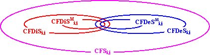
(8)	CJDiS^M_i,j Í CJDiS_i,j Í CJS_i,j and CJDeS^M_i,j Í CJDeS_i,j Í CJS_i,j

that are obviously from the definitions (4)-(6). Figurative, inclusions are:

Fig. 2. Inclusions relations in CJ sets
Note that in generally the sets CJDiS^M_i,j, CJDiS_i,j, CJS_i,j, CJDeS^i,j, CJDeS^M_i,j are not distinct; more, in trees the sets are equals. To prove that the sets CJDiS^M_i,j, CJDiS_i,j, CJS_i,j, CJDeS^i,j, CJDeS^M_i,j are not banal, let’s apply the algorithm (7) to construct sets for graph G from fig. 1. Following example shows that sets CJDiS^M and CJDeS^M are not identically: CJDiS^M_1,2 = {CJ_1,2,[1,2]}; CJ_1,2,[1,2] = {1, 3, 6, 8} CJDiS^M_2,1 = {CJ_2,1,[2,1]}; CJ_2,1,[2,1] = {2, 4, 7} CJDeS^M_1,2 = {CJ_{1,2,[1,3,6,7,4,2]}}; CJ_{1,2,[1,3,6,7,4,2]} = {1} CJDeS^M_1,2 = {CJ_{2,1,[2,4,7,6,3,1]}}; CJ_{2,1,[2,4,7,6,3,1]} = {2} and graphical representation of them are in fig. 3:

Fig. 3. CJDi and CJDe sets for vertices 1 and 2 and graph G from fig. 1
The following example shows that CJDe sets are not included in CJDi sets: CJDiS^M_4,8 = {CJ_{4,8,[4,7,6,8]}}; CJ_{4,8,[4,7,6,8]} = {1, 2, 4, 5} CJDiS^M_8,4 = {CJ_{8,4,[8,6,7,4]}}; CJ_{8,4,[8,6,7,4]} = {8} CJDeS^M_4,8 = {CJ_{4,8,[4,2,1,3,6,8]}}; CJ_{4,8,[4,2,1,3,6,8]} = {4, 5, 7} CJDeS^M_8,4 = {CJ_{8,4,[8,6,3,1,2,4]}}; CJ_{8,4,[8,6,3,1,2,4]} = {8} and graphical representation of them are in fig. 4:

Fig. 4. CJDi_{4,8,[4,7,6,8]} and CJDe_{4,8,[4,2,1,3,6,8]} sets for graph G from fig. 1
The following example shows that sets CJDiS^M can contain more than one set: CJDiS^M_2,8 = {CJ_{2,8,[2,4,7,6,8]} = {1, 2, 5}, CJ_{2,8,[2,1,3,6,8]} = {4, 2, 5}}; CJDiS^M_8,2 = {CJ_{8,2,[8,6,3,1,2]} , CJ_{8,2,[8,6,3,1,2]}}; CJ_{8,2,[8,6,3,1,2]} = CJ_{8,2,[8,6,7,4,2]} = {8}; and graphical representation of them are in fig. 5:

Fig. 5. CJDi_2,8,[24768] and CJDi_2,8,[21368] sets of graph G from fig. 1

4. G_p Subgraph
Let p = (i = v₁, ..., v_l(p) = j) Î P(G) a path starting from vertex i and ending in vertex j. The G_p subgraph of graph G and path p is defined by:

(9)	G_p = (V_p, E_p), V_p = {v Î V : v Ï p\{i, j}}, E_p = {e = (e_a, e_b) Î E : e_a, e_b Ï p\{i, j}}

Note that G_p subgraph associated of graph G and path p is not necessary a connected subgraf, even if G is a connected graph. More, if G is a tree, G_p has at least two connected components. For path p = [1, 3, 5, 4, 7] and graph G from fig. 1 the graph G_{[1, 3, 5, 4, 7]} = G\[1, 3, 5, 4, 7] is not a connected graph. G_p has two connected components: [1, 2] and [7, 6, 8]. Also, from original graph G, p\{1,7} is also a connected component. Using comparison operator ≤ between graphs is obviously that G_p È p ≤ G. In fig. 6 are graphically represented the components of G by path p:

Fig. 6. Graph G, path p = [1, 3, 5, 4, 7], path p\{1, 7} = [3, 5, 4] and subgraph G_p G_p = (V_p, E_p), V_p = {1, 2, 6, 7, 8}, E_p = {(1,2), (6, 7), (6, 8)}
Note that G = G_p È p È [2, 4] È [3, 6].

3. Graph Partitioning in Fragments
Let G = (V, E) be a connected graph and i, j Î V two vertices. Let p Î P(G)_i,j a path from i to j in G.

(10)	CF_i,j,p = {k : k Î V} is named CF fragment of i vs. j and p if: d(G_p)_k,i < d(G_p)_k,j

where subgraph G_p is obtained from graph G and path p according to definition (9). Note that in definition (10) is used term of fragment for CF_i,j,p. Indeed, CF_i,j,p is an fragment, a connected set of vertices from graph G. The set of sets of vertices CFS_i,j = {CF_i,j,p: p Î P(G)_i,j} are named set of CF sets of i vs. j. More, in CFS_i,j,p fragment, there exist the relation:

(11)	" k Î CFS_i,j,p, $ q Î P(G_p)_k.i path from k to i in G_p s. th. q Ç p = {i}

Similar to definitions (5) and (6), CFDi and CFDe fragments are defined:

(12)	CFDi_i,j,p={k : k Î V} is named CFDi fragment of i vs. j and p if: CFDi_i,j,p Î CFS_i,j l(p) = d(G_p)_i,j

The fragments set CFDiS_i,j = {CFDi_i,j,p : p Î P(G)_i,j} are named set of CFDi fragments of i vs. j.

(13)	CFDe_i,j,p={k : k Î V} is named CFDe fragment of i vs. j and p if: CFDe_i,j,p Î CFS_i,j l(p) = δ(G_p)_i,j

The fragments set CFDeS_i,j = {CFDe_i,j,p : p Î P(G)_i,j} are named set of CFDe fragments of i vs. j. CFDi^M_i,j = {f : f Î CFDiS_i,j} is named CFDi^M fragment of i vs. j if l(f) = max{ |cfdi| : cfdi Î CFDiS_i,j}. CFDe^M_i,j = {f : f Î CFDeS_i,j} is named CFDe^M set of i vs. j if l(f) = max{ |cfde| : cfde Î CFDeS_i,j}. The sets CFDi can be constructed as follows:

(14)	CFDi_i,j,p= Æ; CFDi_j,i,p= Æ; For (v = 1; v ≤ \|V\|; v++) If (d(G_p)_v,i < d(G_p)_v,j) then CFDi_i,j,p È = {v}; EndIf; If (d(G_p)_v,j < d(G_p)_v,i) then CFDi_j,i,p È = {v}; EndIf; EndFor;

Note that the algorithm (14) can be applied for any distance operator in place of d(∙), such as detour operator δ(∙). Based on construction (14) the sets CFDi are always fragments. Through CF sets it exist inclusions relations:

(15)	CFDiS^M_i,j Í CFDiS_i,j Í CFS_i,j and CFDeS^M_i,j Í CFDeS_i,j Í CFS_i,j

that are obviously from the definitions (11)-(13). Figurative, inclusions are:

Fig. 7. Inclusions relations for CF sets
Note that in generally the sets CF are not distinct. In trees are even equals. To prove that the sets CFDiS^M_i,j, CFDiS_i,j, CFS_i,j, CFDeS^i,j, CFDeS^M_i,j are not banal, let’s apply the algorithm (14) to construct sets for graph G from fig. 1. Following example shows that sets CFDiS^M and CFDeS^M are not identically: CFDiS^M_1,2 = {CF_1,2,[1,2]}; CF_1,2,[1,2] = {1, 3, 6, 8} CFDiS^M_2,1 = {CF_2,1,[2,1]}; CF_2,1,[2,1] = {2, 4, 7} CFDeS^M_1,2 = {CF_{1,2,[1,3,6,7,4,2]}}; CF_{1,2,[1,3,6,7,4,2]} = {1} CFDeS^M_1,2 = {CF_{2,1,[2,4,7,6,3,1]}}; CF_{2,1,[2,4,7,6,3,1]} = {2} and graphical representation of them are in fig. 3:

Fig. 8. CFDi_1,2,[1,2] and CFDi_{1,2,[1,2,6,7,4,2]} fragments of graph G from fig. 1
The following example shows that CFDe sets are not included in CFDi sets: CFDiS^M_4,8 = {CF_{4,8,[4,7,6,8]}}; CF_{4,8,[4,7,6,8]} = {1, 2, 3, 4, 5}; CFDeS^M_4,8 = {CF_{4,8,[4,2,1,3,6,8]}}; CF_{4,8,[4,2,1,3,6,8]} = {4, 5, 7}; CFDiS^M_8,4 = {CF_{8,4,[8,6,7,4]}} = {{8}} = {CF_{8,4,[8,6,3,1,2,4]}} = CFDeS^M_8,4 and fragments are depicted in fig. 9:

Fig. 9. CFDi_{4,8,[4,7,6,8]} and CFDe_{4,8,[4,2,1,3,6,8]} fragments of graph G from fig. 1
The following example shows that sets CFDiS^M can contain more than one fragment: CFDiS^M_7,1 = {CF_{7,1,[7,4,2,1]} , CF_{7,1,[7,6,3,1]}}; CF_{7,1,[7,4,2,1]} = {6, 7, 8}; CF_{7,1,[7,6,3,1]} = {4, 5, 7} and graphical representation of them are in fig. 10:

Fig. 10. CFDi_{7,1,[7,4,2,1]} and CFDi_{7,1,[7,6,3,1]} fragments of graph G from fig. 1 The Szeged (SzDi) fragments are defined by:

(16)	SzDi_i,j = {k : k Î V} is named SzDi fragment of i vs. j if: d(G)_k,i < d(G)_k,j

The SzDi sets are connected subgraphs (fragments). Looking at (5) and (16) definitions, is easy to observe that:

(17)	CJDi Í SzDi,

and also:

(18)	CFDi Ë SzDi,

The following construction collects the fragments SzDi for all i and j pairs of vertices:

(19)

For (i = 1; i < |X|; i++)

For

_i,j

_j,i

For

and

then

dvi = k;

EndIf

and

then

dvj = k;

EndIf

EndFor

then

_i,j

EndIf

then

_j,i

EndIf

EndFor

EndFor;

A graphical example of SzDi fragments for vertices 2 and 6 and graph G from fig. 1 is depicted in fig. 11:

Fig. 11. SzDi_2,6 and SzDi_6,2 fragments of graph G from fig. 1
Like CJ and CF, SzDe sets can be defined as:

(20)	SzDi_i,j = {k : k Î V} is named SzDe set of i vs. j if: δ(G)_k,i < δ(G)_k,j

SzDe sets are not fragments (connected subgraphs). An example is depicted in fig. 12:

Fig. 12. SzDe_2,6 = {2,3} and SzDe_6,2 = {4, 6, 8} sets for graph G from fig. 1

4. A Comparison between Graph Partitioning Methods
Let us to consider the graph from fig. 13. If CFDi, CJDi and SzDi partitioning methods are applied for graph G from fig. 13 and (1,4) pair of vertices, we have: CFDi_{1,4,[1,2,3,4]} = {1, 8, 9, 10}; CFDi_{4,1,[4,3,2,1]} = {4, 5, 6, 7}; CJDi_{1,4,[1,2,3,4]} = {1, 9, 10}; CJDi_{4,1,[4,3,2,1]} = {4, 5, 6, 7, 8}; SzDi_1,4 = {1, 2, 9, 10}, SzDi_4,1 = {3, 4, 5, 6, 7, 8}.

Fig. 13. Graph G = (V, E); V = {1, ..., 10}; E = {(i, i+1) : 1 ≤ i ≤ 10} È {(10, 1), (8, 3)} and CFDi_{1,4,[1,2,3,4]}, CFDi_{4,1,[4,3,2,1]}, CJDi_{1,4,[1,2,3,4]}, CJDi_{4,1,[4,3,2,1]}, SzDi_1,4, SzDi_4,1 sets
From fig. 13, some conclusions are immediate:

The sets CFDi and CJDi are distinct: CF_{4,1,[4,3,2,1]} Ì CJ_{4,1,[4,3,2,1]} and CF_{1,4,[1,2,3,4]} Ì CJ_{1,4,[1,2,3,4]};

The sets SzDi and CJDi are distinct: CJ_{4,1,[4,3,2,1]} Ì Sz_4,1 and CJ_{1,4,[1,2,3,4]} Ì Sz_1,4;

The sets SzDi and CFDi are distinct: CF_{4,1,[4,3,2,1]} Ì Sz_4,1 and CF_{1,4,[1,2,3,4]} Ë Sz_1,4;

The sets CFDi are not contained in sets SzDi: CF_{4,1,[4,3,2,1]} Ì Sz_4,1 and CF_{1,4,[1,2,3,4]} Ë Sz_1,4;

The CJDi sets are contained in SzDi sets: CJ_{4,1,[4,3,2,1]} Ì Sz_4,1 and CJ_{1,4,[1,2,3,4]} Ì Sz_1,4;
Let us consider another two fragmentation methods, the minimal set that contain i vertex and not contain j vertex MI_i,j:

(21)	MI_i,j = {i}

and maximal set that contain i vertex and not contain j vertex:

(22)	MA_i,j = G\{j}

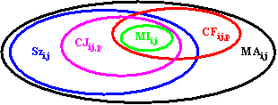
Some interesting properties are also available now:

MI_i,j is a set that is contained in all sets generated for (i,j) pair of vertices:

(23)	MI_i,j Í CJ_i,j,p; MI_i,j Í CF_i,j,p; MI_i,j Í Sz_i,j

MA_i,j it contain all fragments generated for (i,j) pair of vertices:

(24)	CJ_i,j,p Ê MA_i,j; CF_i,j,p Ê MA_i,j; Sz_i,j Ê MA_i,j

The inclusions and intersections of sets are depicted in fig. 14:

Fig. 14. Inclusions between MI, CJ, CF, SZ and MA sets

5. Graph Edges Coloring
The edges of a graph can be colored depending on which fragment are included. To apply the coloring process, is necessary to decompose the graph into connected fragments. From presented methods, connected subgraphs are obtained for CFDi, CFDe and SzDi criteria. The CFDi criterion partition a graph G for a pair of vertices (i, j) into four regions:

region of i’s belonging versus j, that is CFDi_i,j,p;

region of j’s belonging versus i, that is CFDi_j,i,p;

the path p\{i, j};

indifferent region G\{p\{i, j} È CFDi_i,j,p È CFDi_j,i,p}
An important observation is that first three regions are connected sets of vertices (fragments) and last one (indifferent region) it can be a disconnected subgraph. In fig. 15 are depicted partitioning of graph G from fig. 1 into four regions:

Fig. 15. Graph G from fig. 1 edges coloring in two cases: (3, 6) and (3,4) pairs of vertices yellow: CFDi_i,j; turquoise: CFDi_j,i; pink: p\{i, j}; red: rest;
The fragments from fig. 15 are: CFDi_3,6,[3,6] = [1,2,3,5]; CFDi_6,3,[6,3] = [6,7,8]; CFDi_3,4,[3,5,4] = [1,3,6,8]; CFDi_4,3,[4,5,3] = [2,4,7]; Note that for (3,4) pair of vertices, the remaining zone of graph, {(1, 2, 6, 7), (1, 2), (6, 7)} are not connected one. With a similar deduction, The CFDe criterion partition a graph G for a pair of vertices (i, j) into four regions:

region of i’s belonging versus j, that is CFDe_i,j,p;

region of j’s belonging versus i, that is CFDe_j,i,p;

the path p\{i, j};

indifferent region G\{p\{i, j} È CFDe_i,j,p È CFDe_j,i,p}
An important observation is that first three regions are connected sets of vertices (fragments) and last one (indifferent region) it can be a disconnected subgraph. In fig. 16 are depicted partitioning of graph G from fig. 1 into four regions:

Fig. 16. Graph G from fig. 1 edges coloring in two cases: (3, 6) and (3,4) pairs of vertices yellow: CFDe_i,j; turquoise: CFDe_j,i; pink: p\{i, j}; red: rest;
The fragments from fig. 16 are: CFDi_{3,6,[3,1,2,4,7,6]} = [3,5]; CFDi_{6,3,[6,7,4,2,1,3]} = [6,8]; CFDi_{3,4,[3,1,2,4]} = [3,6,8]; CFDi_{4,3,[4,2,1,3]} = [4,7]; Note that for (3,4) pair of vertices, the remaining zone of graph, {(1, 2, 6, 7), (1, 2), (6, 7)} are not connected one. With a similar deduction, The SzDi criterion partition a graph G for a pair of vertices (i, j) into three regions:

region of i’s belonging versus j, that is CFDe_i,j,p;

region of j’s belonging versus i, that is CFDe_j,i,p;

the equidistant region {k : d(k,i) = d(k,j)}.
An important observation is that first two regions are connected sets of vertices (fragments) and last one (equidistant region) it can be a disconnected subgraph. In fig. 17 are depicted partitioning of graph G from fig. 1 into three regions:

Fig. 17. Graph G from fig. 1 edges coloring in two cases: (3, 6) and (3,4) pairs of vertices yellow: CFDe_i,j; turquoise: CFDe_j,i; red: equidistant region {k : d(k,i) = d(k,j)};
The fragments from fig. 17 are: SzDi_3,6 = [1,2,3,5]; SzDi_6,3 = [6,7,8]; SzDi_3,4 = [1,3,6,8]; SzDi_4,3 = [2,4,7];

6. Theoretical Results (Theorems)
Theorem 1. CF is a fragment.
" i, j Î V,  p Î P(G)_i,j path in G from i to j then F_i,j,p fragment
Demonstration:

Fig. 18. Auxiliary construction for theorem 1 demonstration
Let v Î CF_i,j,p. Then:
(Case 1) d(G_p)_v,i < ¥ , d(G_p)_v,j = ¥ and respectively
(Case2) d(G_p)_v,i < ¥ , d(G_p)_v,j < ¥ , d(G_p)_v,i < d(G_p)_v,j
(Case 1, demonstration):
d(G_p)_v,i< ¥ Þ $ p_v,i Î P(G_p)_v,i (P(G_p)_k,i¹ Æ). Let k Î p_v,i Þ $ p_k,i Î P(G_p)_k,i (p_k,i Í p_v,i) Þ

(25)	d(G_p)_k,i< ¥ Þ $ p_v,k Î P(G_p)_v,k (p_v,k Í p_v,i)

If d(G_p)_k,j< ¥ Þ $ p_k,j Î P(G_p)_k,j (P(G_p)_k,j¹ Æ). Let w_v,j= p_v,k È p_k,j; w_v,j Î W(G_p)_v,j (W(Gp)_v,j¹ Æ) Þ d(Gp)_v,j £ l(p_v,k) + l(p_k,j) < ¥ contradiction with d(G_p)_v,j= ¥ Þ

(26)	d(G_p)_k,j= ¥

From (25) and (26) Þ k Î CF_i,j,p Þ p_v,i Í CF_i,j,p Þ v connected with i in CF_i,j,p Þ

(27)	CF_i,j,p connected

(Case 2, demonstration):
d(G_p)_v,i< ¥ Þ $ p_v,i Î P(G_p)_v,i s. th. l(p_v,i) = min{l(q), q Î P(G_p)_v,i} (P(G_p)_v,i¹ Æ; l(p_v,i) = d(G_p)_v,i). Let k Î p_v,i Þ

(28)	$ p_k,i Î P(G_p)_k,i (p_k,i Í p_v,i) , $ p_v,k Î P(G_p)_v,k (p_v,k Í p_v,i)

Because a geodesic path can contain only geodesic paths, from (28) it results: l(p_k,i) = d(G_p)_k,i, l(p_v,k) = d(G_p)_v,k , l(p_v,i) = l(p_v,k) + l(p_k,i) Þ d(G_p)_v,i= d(G_p)_v,k+ d(G_p)_k,i d(G_p)_v,j £ d(G_p)_v,k+ d(G_p)_k,j (d(G_p) a metric); (28) Þ d(G_p)_v,j-d(G_p)_v,i £ d(G_p)_k,j- d(G_p)_k,i From d(G_p)_v,i< d(G_p)_v,j Þ 0 <d(G_p)_v,j- d(G_p)_v,i £ d(G_p)_k,j-d(G_p)_k,i and then: d(G_p)_k,i < d(G_p)_k,j Þ k Î CF_i,j,p Þ p_v,i Í CF_i,j,p Þ

(29)	v connected with i in CF_i,j,p Þ CF_i,j,p connected

From (27) and (29) it result that CF_i,j,p is a connected subgraph (q.e.d.).
Theorem 2. SzDi is a fragment.
" i, j Î V then SZDi_i,j fragment
Demonstration:
Let v Î SZDi_i,j. Then d(G)_v,i< ¥ , d(G)_v,j< ¥ , d(G)_v,i< d(G)_v,j (G connected graph). From d(G)_v,i< ¥ Þ $ p_v,i Î P(G)_v,i s. th. l(p_v,i) = min{l(q), q Î P(G)_v,i} (P(G)_v,i¹ Æ; l(p_v,i) = d(G)_v,i). Let k Î p_v,i Þ

(30)	$ p_k,i Î P(G)_k,i (p_k,i Í p_v,i) , $ p_v,k Î P(G)_v,k (p_v,k Í p_v,i)

Because a geodesic path can contain only geodesic paths, from (28) it results: l(p_k,i) = d(G)_k,i, l(p_v,k) = d(G)_v,k , l(p_v,i) = l(p_v,k) + l(p_k,i) Þ d(G)_v,i= d(G)_v,k+ d(G)_k,i d(G)_v,j £ d(G)_v,k+ d(G)_k,j (d(G) a metric); (30) Þ d(G)_v,j- d(G)_v,i £ d(G)_k,j- d(G)_k,i Because d(G)_v,i< d(G)_v,j Þ 0 < d(G)_v,j-d(G)_v,i £ d(G)_k,j-d(G)_k,i and then d(G)_k,i< d(G)_k,j Þ k Î SzDi_i,j Þ p_v,i Í SzDi_i,j Þ v connected with i in SzDi_i,j Þ SzDi_i,j connected subgraph (q.e.d.).
Theorem 3. CJDi sets are contained in SzDi fragments.
CJDi_i,j,p Ì SzDi_i,j
Demonstration:
Let v Î CJDi_i,j,p. According to definition of CJDi set,

d(G)_v,i < d(G)_v,j

(31)

This is (according to the definition of SzDi fragment) a necessary and enough such that v Î SzDi_i,j,p. From here, it result immediately that CJDi_i,j,p Ì SzDi_i,j (q.e.d.).

References
[1] M. V. Diudea, I. Gutman, L. Jäntschi, 'Molecular Topology', Nova Science, Commack, New York, 2002.
[2] X. Liu, K. Balasubramanian, E. M. Munk, 'Computational Techniques for Vertex Partitioning of Graphs', J. Chem. Comput. Sci., 30 (1990), 263-269.
[3] A. V. Skorobogatov, A. A. Dobrynin, 'Metric Analysis of Graphs', Commun. Math. Comput. Chem., 23 (1988), 105-151.
[4] T. Quenell, 'Eigenvalue comparisons in Graph Theory', Pacific J. of Math., 176-2 (1996), 443-461.
[5] F. Harary, A. J. Schwenk, 'The Spectral Approach to Determining the Number of Walks in a Graph', Pacific J. of Math., 80-2 (1979), 443-449.
[6] S.-Y. Cheng, 'Eigenvalue Comparison Theorems and Its Geometric Applications', Math. Z., 143 (1975), 289-297.
[7] C. S. Basak, R. V. Magnusson, G. Niemi, R. Regal, 'Determining Structural Similarity of Chemicals Using Graph-Theoretic Indices', Discr. Appl. Math., 19 (1988), 17-44.
[8] X. Liu, K. Balasubramanian, E. M. Munk, 'Computational Techniques for Vertex Partitioning of Graphs', J. Chem. Inf. Comput. Sci., 30 (1990), 263-269.
[9] M. Bersohn, 'A Matrix Method for Partitioning the Atoms of a Molecule Into Equivalence Classes', Comput. Chem., 11 (1987), 67-72.
[10] A. T. Balaban, 'Local versus Global (i.e. Atomic versus Molecular) Numerical Modelling of Molecular Graphs', J. Chem. Inf. Comput. Sci., 34 (1994), 398-402.
[11] M. Lerman, I. R. Soare, 'd-Simple Sets, Small Sets and Degree Classes', Pacific J. of Math., 87-1 (1980), 135-155.
[12] D. Dhar, 'Asymptotic Enumeration of Partially Ordered Sets', Pacific J. of Math., 90-2 (1980), 299-306.
[13] A. A. Dobrynin, 'Degeneracy of Some Matrix Graph Invariants', J. of Math. Chem., 14 (1993) 175-184.
[14] A. A. Dobrynin, 'Cubic Graphs with 62 Vertices Having the Same Path Layer Matrix', J. Graph Theory, 17 (1993), 1-4.
[15] A. T. Balaban, 'Applications of Graph Theory in Chemistry', J. Chem. Inf. Comput. Sci., 25 (1985), 334-343.
[16] A. T. Balaban, 'Solved and Unsolved Problems in Chemical Graph Theory', Annals of Discr. Math., 55 (1993), 109-126.
[17] A. A. Dobrynin, A. A. Kochetova, 'Degree Distance of a Graph: A Degree Analogue of the Wiener Index', J. Chem. Inf. Comput. Sci., 36 (1996), 1082-1086.
[18] M. V. Diudea, 'Layer Matrices in Molecular Graphs', J. Chem. Inf. Comput. Sci., 34 (1994), 1064-1071.
[19] M. V. Diudea, M. Topan, A. Graovac, 'Layer Matrices of Walk Degrees', J. Chem. Inf. Comput. Sci., 34 (1994), 1072-1078.
[20] M. Randić, 'Design of Molecules with Desired Properties (A Molecular Similarity Approach to Property Optimization),' in 'Concept and Applications of Molecular Similarity', Ed. A. M. Johnson, G. M. Maggiora, John Wiley & Sons, 5 (1990), 77-145.

Issue 01, p. 37-52

Graph Theory. 2. Vertex Descriptors and Graph Coloring
Lorentz JÄNTSCHI
Technical University of Cluj-Napoca
http://lori.academicdirect.ro

Abstract
This original work presents the construction of a set of ten sequence matrices and their applications for ordering vertices in graphs. For every sequence matrix three ordering criteria are applied: lexicographic ordering, based on strings of numbers, corresponding to every vertex, extracted as rows from sequence matrices; ordering by the sum of path lengths from a given vertex; and ordering by the sum of paths, starting from a given vertex. We also examine a graph that has different orderings for the above criteria. We then proceed to demonstrate that every criterion induced its own partition of graph vertex. We propose the following theoretical result: both LAVS and LVDS criteria generate identical partitioning of vertices in any graph. Finally, a coloring of graph vertices according to introduced ordering criteria was proposed.
Keywords
Graph theory, Vertex descriptors, Matrix based descriptors, Invariants, Graph coloring, Graph partitioning.

1. Introduction
The problem of vertex partitioning in graphs can be solved in different ways [1],[2]. The most frequently used discriminating criteria are well-known square matrices that collect contributions of pairs of vertices from the graph. The adjacency matrix is the simplest matrix of this type. Some authors use characteristic polynomial and its eigenvalue to characterize a given graph [3]. The sequence of eigenvalues forms the graph spectrum [4]. A basic result in spectral geometry is the theorem of Cheng [5]. Let us consider a sequence matrix. It is of dimension n×(n-1), where n is the number of vertices. Such a matrix can be used to compare different graphs (interstructural similarity), when analyzing the columns of sequence matrices, the sums by columns or global sums (generic indices) [6]. It is also possible to compare the vertices of a graph (intrastructural similarity), when analyzing the rows of sequence matrices and the sums by rows [7],[8]. With this observation, a sequence matrix is an elegant method to investigate graphs [9]. Note that the ordering of graph vertices by using sequence matrices is of a partially ordered type [10],[11]. Prior, Dobrynin reported the degeneracy of some sequence matrices [12],[13]. Decomposition of graphs into congruent factors has interesting chemical implications [14],[15]. Dobrynin [16] and Diudea [17],[18] reported distance degree sequences (DPS in our notation) and their chemical applications. The path sequence matrix (APS in our notation) is calculated in order to study molecular similarity [19].

2. Theoretical Considerations
Some definitions are required. Let G = (V, E) be an un-oriented graph. We are note the set of all path in G with P(G). The distance from i to j in G is d(G)_i,j and detour is δ(G)_i,j. For p Î P(G), l(p) denotes the length of path p. t = (v_i)_1≤i≤n is a terminal path if: (1) t Î P(G) and (2) " v Î V s. th. (v_n, v) Î E then t È (v_n, v) Ï P(G). The set of terminal paths starting with i in G is T(G)_i = {t = (v_i)_1≤i≤n s. th. v₁ = i and t terminal path}. The set of terminal paths in G is T(G) = (T(G)_v)_v
Î
V. The set of distance paths from i to j in G is DP(G)_i,j = {p=(x_i)_1
£
i
£
n s. th. p Î P(G), x₁=i, x_n=j & l(p)=d(G)_i,j}. The set of distance path in G is DP(G) = {p = (x_i)_1
£
i
£
n s. th. p Î P(G) and l(p) = }. The set of detour paths from i to j in G is ΔP(G)_i,j = {p=(x_i)_1
£
i
£
n s. th. p Î P(G), x₁=i, x_n=j & l(p)=δ(G)_i,j}. The set of detour path in G is ΔP(G) = {p = (x_i)_1
£
i
£
n s. th. p Î P(G) and l(p) = }. The set of distance terminal paths from i to j in G is DT(G)_i,j = {t=(x_i)_1
£
i
£
n s. th. t Î T(G), x₁=i, x_n=j & l(t)=d(G)_i,j}. The set of distance terminal path in G is DT(G) = {t = (x_i)_1
£
i
£
n s. th. t Î T(G) and l(t) = }. The set of detour terminal paths from i to j in G is ΔT(G)_i,j = {t=(x_i)_1
£
i
£
n s. th. t Î T(G), x₁=i, x_n=j & l(t)= δ(G)_i,j}. The set of detour terminal path in G is ΔT(G) = {t = (x_i)_1
£
i
£
n s. th. t Î T(G) and l(t) = }. Note that if G = (V, E) is a connected graph, then " v Î V, " e Î E $ t Î T(G)_v s. th. e Í t. Thus, any connected graph can be reconstructed from the terminal path list starting from an arbitrary vertex. Also, " i, j Î V, T(G)_j can be constructed from T(G)_i. Consequently, the sets of terminal paths T(G)_v, v Î V are equivalent by construction. In order to generate sequence matrices, we compute terminal paths. Let G = (V, E), V = {1, …, 8}, E = {(1, 2), (1, 3), (2, 4), (3, 5), (3, 6), (4, 5), (4, 7), (6, 7), (7,8)} shown in figure 1:

Fig. 1. Graph G (see above)
We have devised a 16-bit windows original computer program to list all terminal paths. For the graph in figure 1, we have obtained the following set of terminal paths for vertex 1:

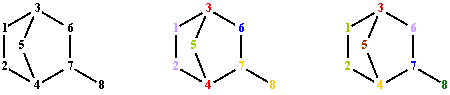
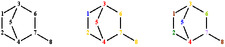
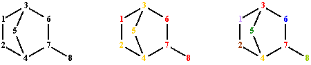
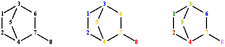
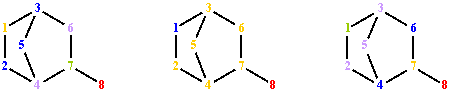
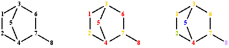
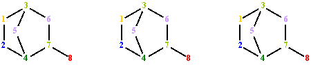
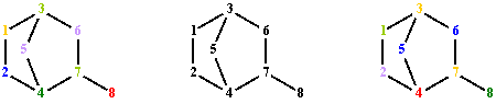
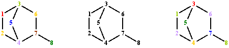
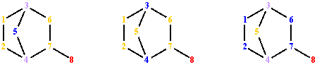
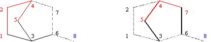
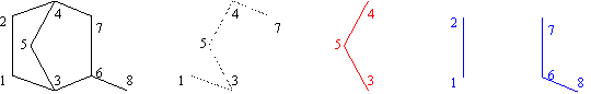
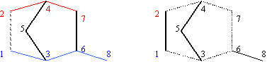
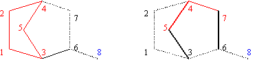
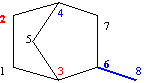
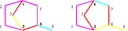
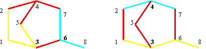
T(G)₁
1 2 4 5 3 6 7 8
1 2 4 7 8
1 2 4 7 6 3 5
1 3 6 7 8
1 3 6 7 4 2
1 3 6 7 4 5
1 3 5 4 7 6
1 3 5 4 7 8
1 3 5 4 2

Fig. 2. Terminal paths of graph G from fig. 1 starting from vertex 1

3. The Construction of Sequence Matrices of Numbering
We extend the concept used for the distance degree sequence matrix [16] and layer path (path degree sequence) [19] matrix to construct a set of 10 sequence matrices. A sequence matrix is a matrix that collects vertex contribution in each row and elongation of paths in each column. The elements of the matrix cumulate a value of vertex property for a given elongation. Sequence matrices are of dimension n×(n-1) and are given by following definitions: SMN (sequence matrix of numbering) of paths (P) which starts with i and has length j is APS(G)_i,j = |{p Î P(G), s. th. p₁ = i, l(p) = j}|, where p₁ is the first vertex from path p and operator |∙| is the cardinal operator. SMN of distance P that starts with i and has length j is DPS(G)_i,j = |{p Î APS(G)_i,j, s. th. p Î DP(G)}|. SMN of detour P that starts with i and has length j is ΔPS(G)_i,j = |{p Î APS(G)_i,j, s. th. p Î ΔP(G)}|. SMN of terminal paths (T) which starts with i and has length j is ATS(G)_i,j = |{t Î T(G), s. th. t₁ = i, l(t) = j}}|. SMN of distance T that starts with i and has length j is DTS(G)_i,j = |{p Î ATS(G)_i,j, s. th. p Î DT(G)}|. SMN of detour T that starts with i and has length j is ΔTS(G)_i,j = |{p Î ATS(G)_i,j, s. th. p Î ΔT(G)}|. SMN of the vertex situated at the end of paths that starts with i and has j edges is AVS(G)_i,j = |{v Î V, s. th. $ p Î P(G), p₁ = i, p_j+1 = v, l(p) = j}|. SMN of the vertex situated at the end of distance paths that starts with i and has j edges is DVS(G)_i,j = |{v Î V, s. th. $ p Î DP(G), p₁= i, p_j+1= v, l(p)=j}|. SMN of the vertex situated at the end of detour paths that starts with i and has j edges is ΔVS(G)_i,j = |{v Î V, s. th. $ p Î ΔP(G), p₁ = i, p_j+1 = v, l(p)=j}|. SMN of the cycles that contain vertex i and has j edges is ACS(G)_i,j = |{p Î P(G), s. th. l(p) = j-1 and (p_j,p₁) Î E}|. If an lexicographically ordering are applied to the sequence matrices of numbering (SMN), through permutation of one line with another, and the new matrix obtained can be used to make interstructural comparisons (with any other graph) because a lexicographically ordered matrix is independent with respect to labeling. When two vertices are compared, lexicographic ordering is also useful from the point of view of the selected criterion. The results of lexicographic ordering can be used to index the graph, by permuting the old indexing. The computer program used in lexicographic ordering (quicksort method), gives permutation of partial ordering (σ in what follows). Ten sequence matrices, ten lexicographically associated matrices and ten permutations σ are computed. Two vertex indices in every case (from ten cases) are calculated. The first is sum of elements from the row (the number of total paths), the second is the weighted sum of elements from the row (the length of total paths). For the graph G from figure 1 we obtain a set of ten tables with three different ordering criteria (table 1-10).
Table 1. APS and LAPS numbered sequences

APS	1	2	3	4	5	6	7	Σ_iS_i,j	Σ_iS_i,j∙i	LAPS	1	2	3	4	5	6	7	Σ_iS_i,j	Σ_iS_i,j∙i
1	2	3	4	7	6	2	1	25	97	1=σ(8)	1	2	3	4	5	5	2	22	99
2	2	3	5	5	6	4	0	25	97	2=σ(1)	2	3	4	7	6	2	1	25	97
3	3	3	5	7	3	0	0	21	67	3=σ(2)	2	3	5	5	6	4	0	25	97
4	3	4	4	6	3	1	0	21	68	4=σ(6)	2	4	4	5	6	3	0	24	90
5	2	4	5	5	4	5	1	26	102	5=σ(5)	2	4	5	5	4	5	1	26	102
6	2	4	4	5	6	3	0	24	90	6=σ(7)	3	3	4	5	5	2	0	22	78
7	3	3	4	5	5	2	0	22	78	7=σ(3)	3	3	5	7	3	0	0	21	67
8	1	2	3	4	5	5	2	22	99	8=σ(4)	3	4	4	6	3	1	0	21	68

Table 2. DPS and LDPS numbered sequences

DPS	1	2	3	4	5	6	7	Σ_iS_i,j	Σ_iS_i,j∙i	LDPS	1	2	3	4	5	6	7	Σ_iS_i,j	Σ_iS_i,j∙i
1	2	3	2	2	0	0	0	9	22	1=σ(8)	1	2	3	2	0	0	0	8	22
2	2	3	3	0	0	0	0	8	17	2=σ(1)	2	3	2	2	0	0	0	9	22
3	3	3	1	0	0	0	0	7	12	3=σ(2)	2	3	3	0	0	0	0	8	17
4	3	4	0	0	0	0	0	7	11	4=σ(5)	2	4	1	0	0	0	0	7	13
5	2	4	1	0	0	0	0	7	13	5=σ(6)	2	4	2	0	0	0	0	8	16
6	2	4	2	0	0	0	0	8	16	6=σ(3)	3	3	1	0	0	0	0	7	12
7	3	3	2	0	0	0	0	8	15	7=σ(7)	3	3	2	0	0	0	0	8	15
8	1	2	3	2	0	0	0	8	22	8=σ(4)	3	4	0	0	0	0	0	7	11

Table 3. ΔPS and LΔPS numbered sequences

ΔPS	1	2	3	4	5	6	7	Σ_iS_i,j	Σ_iS_i,j∙i	LΔPS	1	2	3	4	5	6	7	Σ_iS_i,j	Σ_iS_i,j∙i
1	0	0	0	1	4	2	1	8	43	1=σ(1)	0	0	0	1	4	2	1	8	43
2	0	0	0	1	4	4	0	9	48	2=σ(6)	0	0	0	1	4	3	0	8	42
3	0	0	2	4	3	0	0	9	37	3=σ(2)	0	0	0	1	4	4	0	9	48
4	0	0	2	4	2	1	0	9	38	4=σ(5)	0	0	0	4	0	4	1	9	47
5	0	0	0	4	0	4	1	9	47	5=σ(4)	0	0	2	4	2	1	0	9	38
6	0	0	0	1	4	3	0	8	42	6=σ(3)	0	0	2	4	3	0	0	9	37
7	1	0	0	1	4	2	0	8	37	7=σ(8)	1	0	0	0	1	4	2	8	44
8	1	0	0	0	1	4	2	8	44	8=σ(7)	1	0	0	1	4	2	0	8	37

Table 4. ATS and LATS numbered sequences

ATS	1	2	3	4	5	6	7	Σ_iS_i,j	Σ_iS_i,j∙i	LATS	1	2	3	4	5	6	7	Σ_iS_i,j	Σ_iS_i,j∙i
1	0	0	0	3	4	1	1	9	45	1=σ(8)	0	0	0	0	1	3	2	6	37
2	0	0	1	1	3	4	0	9	46	2=σ(1)	0	0	0	3	4	1	1	9	45
3	0	0	1	5	3	0	0	9	38	3=σ(5)	0	0	1	1	0	4	1	7	38
4	0	1	0	3	2	1	0	7	30	4=σ(2)	0	0	1	1	3	4	0	9	46
5	0	0	1	1	0	4	1	7	38	5=σ(3)	0	0	1	5	3	0	0	9	38
6	0	1	0	0	3	3	0	7	35	6=σ(6)	0	1	0	0	3	3	0	7	35
7	1	0	0	1	3	2	0	7	32	7=σ(4)	0	1	0	3	2	1	0	7	30
8	0	0	0	0	1	3	2	6	37	8=σ(7)	1	0	0	1	3	2	0	7	32

Table 5. DTS and LDTS numbered sequences

DTS	1	2	3	4	5	6	7	Σ_iS_i,j	Σ_iS_i,j∙i	LDTS	1	2	3	4	5	6	7	Σ_iS_i,j	Σ_iS_i,j∙i
1	0	0	0	2	0	0	0	2	8	1=σ(8)	0	0	0	0	0	0	0	0	0
2	0	0	1	0	0	0	0	1	3	2=σ(1)	0	0	0	2	0	0	0	2	8
3	0	0	1	0	0	0	0	1	3	3=σ(3)	0	0	1	0	0	0	0	1	3
4	0	1	0	0	0	0	0	1	2	4=σ(5)	0	0	1	0	0	0	0	1	3
5	0	0	1	0	0	0	0	1	3	5=σ(2)	0	0	1	0	0	0	0	1	3
6	0	1	0	0	0	0	0	1	2	6=σ(4)	0	1	0	0	0	0	0	1	2
7	1	0	0	0	0	0	0	1	1	7=σ(6)	0	1	0	0	0	0	0	1	2
8	0	0	0	0	0	0	0	0	0	8=σ(7)	1	0	0	0	0	0	0	1	1

Table 6. ΔTS and LΔTS numbered sequences

ΔTS	1	2	3	4	5	6	7	Σ_iS_i,j	Σ_iS_i,j∙i	LΔTS	1	2	3	4	5	6	7	Σ_iS_i,j	Σ_iS_i,j∙i
1	0	0	0	0	2	1	1	4	23	1=σ(8)	0	0	0	0	0	2	2	4	26
2	0	0	0	0	1	4	0	5	29	2=σ(5)	0	0	0	0	0	3	1	4	25
3	0	0	0	2	3	0	0	5	23	3=σ(6)	0	0	0	0	1	3	0	4	23
4	0	0	0	2	1	1	0	4	19	4=σ(2)	0	0	0	0	1	4	0	5	29
5	0	0	0	0	0	3	1	4	25	5=σ(1)	0	0	0	0	2	1	1	4	23
6	0	0	0	0	1	3	0	4	23	6=σ(4)	0	0	0	2	1	1	0	4	19
7	1	0	0	0	2	2	0	5	23	7=σ(3)	0	0	0	2	3	0	0	5	23
8	0	0	0	0	0	2	2	4	26	8=σ(7)	1	0	0	0	2	2	0	5	23

Table 7. AVS and LAVS numbered sequences

AVS	1	2	3	4	5	6	7	Σ_iS_i,j	Σ_iS_i,j∙i	LAVS	1	2	3	4	5	6	7	Σ_iS_i,j	Σ_iS_i,j∙i
1	3	6	7	8	8	8	8	48	212	1=σ(8)	2	4	7	8	8	8	8	45	207
2	3	6	8	8	8	8	8	49	215	2=σ(1)	3	6	7	8	8	8	8	48	212
3	4	7	8	8	8	8	8	51	218	3=σ(2)	3	6	8	8	8	8	8	49	215
4	4	8	8	8	8	8	8	52	220	4=σ(5)	3	7	8	8	8	8	8	50	217
5	3	7	8	8	8	8	8	50	217	5=σ(6)	3	7	8	8	8	8	8	50	217
6	3	7	8	8	8	8	8	50	217	6=σ(3)	4	7	8	8	8	8	8	51	218
7	4	7	8	8	8	8	8	51	218	7=σ(7)	4	7	8	8	8	8	8	51	218
8	2	4	7	8	8	8	8	45	207	8=σ(4)	4	8	8	8	8	8	8	52	220

Table 8. DVS and LDVS numbered sequences

DVS	1	2	3	4	5	6	7	Σ_iS_i,j	Σ_iS_i,j∙i	LDVS	1	2	3	4	5	6	7	Σ_iS_i,j	Σ_iS_i,j∙i
1	2	3	1	1	0	0	0	7	15	1=σ(8)	1	2	3	1	0	0	0	7	18
2	2	3	2	0	0	0	0	7	14	2=σ(1)	2	3	1	1	0	0	0	7	15
3	3	3	1	0	0	0	0	7	12	3=σ(2)	2	3	2	0	0	0	0	7	14
4	3	4	0	0	0	0	0	7	11	4=σ(5)	2	4	1	0	0	0	0	7	13
5	2	4	1	0	0	0	0	7	13	5=σ(6)	2	4	1	0	0	0	0	7	13
6	2	4	1	0	0	0	0	7	13	6=σ(3)	3	3	1	0	0	0	0	7	12
7	3	3	1	0	0	0	0	7	12	7=σ(7)	3	3	1	0	0	0	0	7	12
8	1	2	3	1	0	0	0	7	18	8=σ(4)	3	4	0	0	0	0	0	7	11

Table 9. ΔVS and LΔVS numbered sequences

ΔVS	1	2	3	4	5	6	7	Σ_iS_i,j	Σ_iS_i,j∙i	LΔVS	1	2	3	4	5	6	7	Σ_iS_i,j	Σ_iS_i,j∙i
1	0	0	0	1	3	2	1	7	38	1=σ(1)	0	0	0	1	3	2	1	7	38
2	0	0	0	1	3	3	0	7	37	2=σ(2)	0	0	0	1	3	3	0	7	37
3	0	0	1	3	3	0	0	7	30	3=σ(6)	0	0	0	1	3	3	0	7	37
4	0	0	1	3	2	1	0	7	31	4=σ(5)	0	0	0	2	0	4	1	7	39
5	0	0	0	2	0	4	1	7	39	5=σ(4)	0	0	1	3	2	1	0	7	31
6	0	0	0	1	3	3	0	7	37	6=σ(3)	0	0	1	3	3	0	0	7	30
7	1	0	0	1	3	2	0	7	32	7=σ(8)	1	0	0	0	1	3	2	7	38
8	1	0	0	0	1	3	2	7	38	8=σ(7)	1	0	0	1	3	2	0	7	32

Table 10. ACS and LACS numbered sequences

ACS	1	2	3	4	5	6	7	Σ_iS_i,j	Σ_iS_i,j∙i	LACS	1	2	3	4	5	6	7	Σ_iS_i,j	Σ_iS_i,j∙i
1	0	0	0	1	1	0	0	2	11	1=σ(8)	0	0	0	0	0	0	0	0	0
2	0	0	0	1	1	0	0	2	11	2=σ(1)	0	0	0	0	1	1	0	2	11
3	0	0	0	2	1	0	0	3	16	3=σ(2)	0	0	0	0	1	1	0	2	11
4	0	0	0	2	1	0	0	3	16	4=σ(6)	0	0	0	0	1	1	0	2	11
5	0	0	0	2	0	0	0	2	10	5=σ(7)	0	0	0	0	1	1	0	2	11
6	0	0	0	1	1	0	0	2	11	6=σ(5)	0	0	0	0	2	0	0	2	10
7	0	0	0	1	1	0	0	2	11	7=σ(3)	0	0	0	0	2	1	0	3	16
8	0	0	0	0	0	0	0	0	0	8=σ(4)	0	0	0	0	2	1	0	3	16

4. Graph Partitioning
Three operators on SMN matrices were applied for vertex comparison: LSMN (lexicographically ordered matrix of numbering), SMNΣ_pn_p (sum of all path number that satisfy selected criteria) and SMNΣ_pn_p∙l(p) (sum of all length of path that satisfy selected criteria).
Every operator induces a partial ordering in V (the set of vertices form the graph), and partitions the vertices in classes of equivalence that it correspond to equal operator values. For example, 1 is equivalent with 2 by APSΣ_pn_p, with 6,7 and 8 by ΔPSΣ_pn_p, with 2, 6, 7 by ACS and ACSΣ_pn_p∙l(p), with 2, 5, 6, 7 by ACSΣ_pn_p, with 4, 5, 6 and 8 by ΔTSΣ_pn_p.
All vertices are equivalent by ΔVSΣ_pn_p and DVSΣ_pn_p. Vertex 1 is singulary according to APSΣ_pn_p∙l(p), DPSΣ_pn_p, ΔPSΣ_pn_p∙l(p), ATSΣ_pn_p∙l(p), LDTS, DTSΣ_pn_p, DTSΣ_pn_p∙l(p), LAVS, AVSΣ_pn_p, AVSΣ_pn_p∙l(p), LDVS, DVSΣ_pn_p∙l(p) and LΔVS.
This example demonstrates the flexibility of sequence matrix criteria in the characterization of various properties of vertices. Let us look at all partial orderings induced in the graph by every sequence matrix.
LAPS discriminates all vertices for the graph in fig. 1.
The values obtained by applying Σ_pn_p and Σ_pn_p∙l(p) operators are degenerate in the case of APS.

APSΣ_pn_p partitioning V(G) in 5 classes of equivalence: P(V(G), APSΣ_pn_p) = {(3,4), (7,8), (6), (1,2), (5)}.

APSΣ_pn_p∙l(p) partitions V(G) in 7 classes of equivalence: P(V(G), APSΣ_pn_p∙l(p)) = {(7), (8), (6), (4), (2,3), (1), (5)}.
LDPS discriminates all vertices for the graph in fig. 1.
The values for Σ_pn_p and Σ_pn_p∙l(p) operators are degenerate in the case of DPS.

DPSΣ_pn_p partitions V(G) in 3 classes of equivalence: P(V(G), DPSΣ_pn_p) = {(3,4,5), (2,6,7,8), (1)}.

DPSΣ_pn_p∙l(p) partitions V(G) in 7 classes of equivalence: P(V(G), DPSΣ_pn_p∙l(p)) = {(8), (6), (4), (7), (5), (3), (1,2)}.
All vertices for the graph from fig. 1 are discriminated by LΔPS criterion.
The values for Σ_pn_p and Σ_pn_p∙l(p) operators are degenerate according to ΔPS criterion.

ΔPSΣ_pn_p partitions V(G) in 2 classes of equivalence: P(V(G), ΔPSΣ_pn_p) = {(1,6,7,8), (2,3,4,5)}.

ΔPSΣ_pn_p∙l(p) partitions V(G) in 7 classes of equivalence: P(V(G), ΔPSΣ_pn_p∙l(p)) = {(3,7), (4), (6), (1), (8), (5), (2)}.
LATS discriminates all vertices for the graph G.
The values for Σ_pn_p and Σ_pn_p∙l(p) are degenerate according to ATS.

ATSΣ_pn_p partitions V(G) in 3 classes of equivalence: P(V(G), ATSΣ_pn_p) = {(8), (4,5,6,7), (1,2,3)}.

ATSΣ_pn_p∙l(p) partitions V(G) in 7 classes of equivalence: P(V(G), ATSΣ_pn_p∙l(p)) = {(4), (7), (6), (8), (3,5), (1), (2)}.
LDTS partitions the vertices of G in 5 classes of equivalence: P(V(G), LDTS) = {(8), (1), (2,3,5), (4,6), (7)}.
The values for Σ_pn_p and Σ_pn_p∙l(p) operators are degenerate according to DTS.

DTSΣ_pn_p partitions V(G) in 3 classes of equivalence: P(V(G), DTSΣ_pn_p) = {(8), (2,3,4,5,6,7), (1)}.

DTSΣ_pn_p∙l(p) partitions V(G) in 5 classes of equivalence: P(V(G), DTSΣ_pn_p∙l(p)) = {(8), (7), (4,6), (2,3,5), (1)}.
LΔTS discriminates all vertices for the graph in fig. 1.
The values for Σ_pn_p and Σ_pn_p∙l(p) operators are degenerate in ΔTS criteria.

ΔTSΣ_pn_p partitions V(G) in 2 classes of equivalence: P(V(G), ΔTSΣ_pn_p) = {(1,4,5,6,8), (2,3,7)}.

ΔTSΣ_pn_p∙l(p) partitions V(G) in 5 classes of equivalence: P(V(G), ΔTSΣ_pn_p∙l(p)) = {(4), (1,3,6,7), (5), (8), (2)}.
LAVS partitions the vertices of G in 6 classes of equivalence: P(V(G), LAVS) = {(8), (1), (2), (5,6), (3,7), (4)}.
The values for Σ_pn_p and Σ_pn_n∙l(p) are degenerate in AVS criteria.

AVSΣ_pn_p partitions V(G) in 6 classes of equivalence: P(V(G), AVSΣ_pn_p) = {(8), (1), (2), (5,6), (3,7), (4)}.

AVSΣ_pn_p∙l(p) partitions V(G) in 6 classes of equivalence: P(V(G), AVSΣ_pn_p∙l(p)) = {(8), (1), (2), (5,6), (3,7), (4)}.
LDVS partitions the vertices of G in 6 classes of equivalence: P(V(G), LDVS) = {(8), (1), (2), (5,6), (3,7), (4)}.
The values for Σ_pn_p and Σ_pn_p∙l(p) are degenerate in DVS criteria.

DVSΣ_pn_p does not discriminate the vertices of G: P(V(G), DVSΣ_pn_p) = {(1,2,3,4,5,6,7,8)}.

DVSΣ_pn_p∙l(p) partitions V(G) in 6 classes of equivalence: P(V(G), DTSΣ_pn_p∙l(p)) = {(4), (3,7), (5,6), (2), (1), (8)}.
LΔVS partitions V(G) in 7 classes of equivalence: P(V(G), LΔVS) = {(1), (2,6), (5), (4), (3), (8), (7)}.
The values for Σ_pn_p and Σ_pn_p∙l(p) operators are totally degenerate in ΔVS criteria.

ΔVSΣ_pn_p partitions does not discriminate the vertices: P(V(G), ΔVSΣ_pn_p) = {(1,2,3,4,5,6,7,8)}.

ΔVSΣ_pn_p∙l(p) partitions V(G) in 6 classes of equivalence: P(V(G), ΔVSΣ_pn_p∙l(p)) = {(3), (4), (7), (2,6), (1,8), (5)}.
LACS partitions V(G) in 4 classes of equivalence: P(V(G), LACS) = {(8), (1,2,6,7), (5), (3,4)}.
The values for Σ_pn_p and Σ_pn_p∙l(p) are degenerate in ACS.

ACSΣ_pn_p partitions V(G) in 3 classes: P(V(G), ACSΣ_pn_p) = {(8), (1,2,5,6,7), (3,4)}.

ACSΣ_pn_p∙l(p) partitions V(G) in 4 classes of equivalence: P(V(G), ACSΣ_pn_p∙l(p)) = {(8), (5), (1,2,6,7), (3,4)}.
Note that the matrices LAVS and LDVS contain different values, but induce the same ordering " σ " for vertices:
σ_LAVS = = σ_LDVS (σP)
The property (σP) was verified by a set of various graphs, with different numbers of cycles, edges and vertices. In each case, the LAVS and LDVS criteria induce the same partial ordering for vertices.

5. Vertices Coloring
According to the partitions induced and presented in tables 1-10 a graph vertices coloring are making. In colorings, a code color was used. In increasing order of values for selected criteria, the colors used are red, gold, blue, lavender, lime, green and brown. For the partitions that discriminate all vertices no coloring was made.

Fig. 3. Graph G vertices colorings from fig. 1; partitions: LAPS, APSΣ_pn_p and APSΣ_pn_p∙l(p)

Fig. 4. Graph G vertices colorings from fig. 1; partitions: LDPS, DPSΣ_pn_p and DPSΣ_pn_p∙l(p)

Fig. 5. Graph G vertices colorings from fig. 1; partitions: LΔPS, ΔPSΣ_pn_p and ΔPSΣ_pn_p∙l(p)

Fig. 6. Graph G vertices colorings from fig. 1; partitions: LATS, ATSΣ_pn_p and ATSΣ_pn_p∙l(p)

Fig. 7. Graph G vertices colorings from fig. 1; partitions: LDTS, DTSΣ_pn_p and DTSΣ_pn_p∙l(p)

Fig. 8. Graph G vertices colorings from fig. 1; partitions: LΔTS, ΔTSΣ_pn_p and ΔTSΣ_pn_p∙l(p)

Fig. 9. Graph G vertices colorings from fig. 1; partitions: LAVS, AVSΣ_pn_p and AVSΣ_pn_p∙l(p)

Fig. 10. Graph G vertices colorings from fig. 1; partitions: LDVS, DVSΣ_pn_p and DVSΣ_pn_p∙l(p)

Fig. 11. Graph G vertices colorings from fig. 1; partitions: LΔVS, ΔVSΣ_pn_p and ΔVSΣ_pn_p∙l(p)

Fig. 12. Graph G vertices colorings from fig. 1; partitions: LACS, ACSΣ_pn_p and ACSΣ_pn_p∙l(p)

6. Conclusions
The analyzed matrix critters are capable to partitioning vertices in equivalence classes by different properties (i.e. number of paths, length of paths, et all). All criteria give a specific partitioning of vertices, excepting LAVS and LDVS ordering. For LAVS and LDVS criterion, an interesting property result: although the individual matrix values are different, comparison rules match, so that the two matrices induce identical partitioning. Testing on a large set of graphs, the partitioning rule LADS ≡ LVDS remain same. That is a subject for a new theorem that will be proved later. More, all AVS criterion (AVSΣ_pn_p and AVSΣ_pn_p∙l(p) and LAVS) make same partitioning of graph vertices for the given graph G from fig. 1. More, the ordering is the same (see fig. 9). Vertex partitioning can be applied in graph coloring [20], the theory of traffic (lights), distributed electric circuits, computer networks [21], and chemical graphs [22]. Edge partitioning is another problem that can be solved using terminal path structure. For more details about this subject, please consult [23].

References
[1]. Liu X., Balasubramanian K., Munk E. M., 'Computational Techniques for Vertex Partitioning of Graphs', J. Chem. Comput. Sci., 30 (1990), 263-269.
[2]. Skorobogatov A. V., Dobrynin A. A., 'Metric Analysis of Graphs', Commun. Math. Comput. Chem., 23(1988), 105-151.
[3]. Quenell T., 'Eigenvalue comparisons in Graph Theory', Pacific J. of Math., 176-2(1996), 443-461.
[4]. Harary F., Schwenk A. J., 'The Spectral Approach to Determining the Number of Walks in a Graph', Pacific J. of Math., 80-2(1979), 443-449.
[5]. Cheng S.-Y., 'Eigenvalue Comparison Theorems and Its Geometric Applications', Math. Z., 143(1975), 289-297.
[6]. Basak C. S., R. V. Magnusson, G. Niemi, R. Regal, 'Determining Structural Similarity of Chemicals Using Graph-Theoretic Indices', Discr. Appl. Math., 19(1988), 17-44.
[7]. Liu X., Balasubramanian K., E. M. Munk, 'Computational Techniques for Vertex Partitioning of Graphs', J. Chem. Inf. Comput. Sci., 30(1990), 263-269.
[8]. Bersohn M., 'A Matrix Method for Partitioning the Atoms of a Molecule Into Equivalence Classes', Comput. Chem., 11(1987), 67-72.
[9]. Balaban A. T., 'Local versus Global (i.e. Atomic versus Molecular) Numerical Modelling of Molecular Graphs', J. Chem. Inf. Comput. Sci., 34(1994), 398-402.
[10]. Lerman M., Soare I. R., 'd-Simple Sets, Small Sets and Degree Classes', Pacific J. of Math., 87-1(1980), 135-155.
[11]. Dhar D., 'Asymptotic Enumeration of Partially Ordered Sets', Pacific J. of Math., 90-2(1980), 299-306.
[12]. Dobrynin A. A., 'Degeneracy of Some Matrix Graph Invariants', J. of Math. Chem., 14(1993) 175-184.
[13]. Dobrynin A. A., 'Cubic Graphs with 62 Vertices Having the Same Path Layer Matrix', J. Graph Theory, 17(1993), 1-4.
[14]. Balaban A. T., 'Applications of Graph Theory in Chemistry', J. Chem. Inf. Comput. Sci., 25(1985), 334-343.
[15]. Balaban A. T., 'Solved and Unsolved Problems in Chemical Graph Theory', Annals of Discr. Math., 55(1993), 109-126.
[16]. Dobrynin A. A., Kochetova A. A., 'Degree Distance of a Graph: A Degree Analogue of the Wiener Index', J. Chem. Inf. Comput. Sci., 36(1996), 1082-1086.
[17]. Diudea M. V., 'Layer Matrices in Molecular Graphs', J. Chem. Inf. Comput. Sci., 34(1994), 1064-1071.
[18]. Diudea M. V., Topan M., Graovac A., 'Layer Matrices of Walk Degrees', J. Chem. Inf. Comput. Sci., 34(1994), 1072-1078.
[19]. Randić M., 'Design of Molecules with Desired Properties (A Molecular Similarity Approach to Property Optimization),' in 'Concept and Applications of Molecular Similarity', Ed. A. M. Johnson, G. M. Maggiora, John Wiley & Sons, 5(1990), 77-145.
[20]. Exoo G., 'Some New Ramsey Colorings', The Electronic J. of Combinatorics, 5(1998), #R29(1-5).
[21]. Jäntschi L., L. M. Ungureşan, 'Special Chapters of Chemistry for Automatics' (in Romanian), U. T. Pres, Cluj-Napoca, Romania, (2001), 1-202.
[22]. Diudea M. V., Gutman I., Jäntschi L., 'Molecular Topology', Nova Science, Huntington, New York, (2001), 1-332.
[23]. Jäntschi L., 'Graph Theory. 1. Fragmentation of Structural Graphs', Leonardo Electronic Journal of Practices and Technologies, 1 (2002), 19-36.

Issue 01, p. 53-60

Loco2000. Technical Characteristics
Gabriel MOISA
Technical University Cluj-Napoca

Abstract
The paper show the function parameters of locomotive components “Loco 2000”, putting accent from their maximal values; the mode who works the force circuit, insisting of modulation technique necessary to obtain a high power factor and to eliminate harmonics. Is described the mode in who are realized the speed regulation and the afferent exploitation data. In the ultimate part of work is presenting the operation mode of the command-control MICAS-S2 system, the different commands imposed to others components (of the force circuit) and, in finale, the three diagnostic levels putting in service in case of troubles in system.
Keywords
Locomotive characteristics, Command systems, Control systems, European railways.

1. Introduction
“Loco 2000”, Re 4/4 460 type, is began in the trans-alpine transport in 1992 year, on the autumn. Is realized under ABB limited, Zurich and respond to very high exigencies, that: high traction force, necessary to surmount big ramps who reach occasionally 27 ‰, a good curve situate and small maintenance necessity. Is concept to generate minimal network troubles, to use fully the regenerative braking, who the denomination “exploitation less of wearing”. The locomotive use on the first the principal automatic circuit breaker with vide, developed by ABB, who no necessitate, practically, no maintenance. She uses frequently the regenerative braking, practically to stop, being a little fault of current on the supply under the route that circulates. Being given the entire exploitations exigency from European railways by 15 kV, 16 2/3 Hz, can be adapted on c.c. network by 3000 V, she can circulate very good in others countries than Switzerland.

2. Technical Description
The commercial exploitation of this type of locomotives is begun in year 1992 in the autumn. They are realized by “ABB Sistèmes de Transport SA” Zurich from cadre of Federal railroads (CFF). Them are in measure to circulate under ramps by 27‰, developing a maxim torque by 192 kN∙m. The maxim torque is available at a speed by 88 km/h, situated in proximity of adherence limit. At maxim technique speed, that is reducing under la 83 kN∙m. In her sequence, the axle power oscillates between 6100 and 4800 kW.

(F-Traction, B-Braking, v-Speed, Z-Axle torque, ZB- Axle braking torque, Zp-Limit of adherence force)
Figure no 1. Torque-speed diagram of locomotive Re 4/4 460
The force electric circuit contents the principal transformer, with four independent traction windings, where are racordate, two by two, the frequency static converters. Hereby, in case of defect of a traction system, the train can continue the race at half-power. The GTO thyristors, with a blockage tension by 4.5 kV and a commutation current by 2.5 kA, permit the exploitation of intermediate converter circuit, in coupling so called in three points, with a nominal tension by 3.5 kV. For high powers, is benefiting a high tension in the intermediate circuit and permit the mention of currents between the admissible limits. She offer, such as, the possibility to use some circuit for two-current locomotives, that circulate at continuum current network by 3000 V. Otherwise, is similar with locomotive ÖBB, series 1822. Grace of triple tension levels (0, 50 and 100%), the three points coupling of intermediate circuit offer the advantage of a bigger approximation of sinusoid. In this case, the request in tension of thyristors is not so big and is not need by a series coupling of semiconductor devices between poles. The traction motors are high speeds, with four poles and the armature in court-circuit. The maxim speed is by 4180 rot/min, with a supply frequency by 143 Hz. The motors power in continuum regime is by 1200 kW, at a tension by 2640 V. The admissible overload is Pmax = 1560 kW. The isolation and leakage inductance are geared to the particular exploitation conditions with inverter, by manner that the supplementary inductance for attenuate of harmonics no be necessary. The locomotive uses the regenerative braking as a prime priority. She serves to maintenance of train speed in descent under pant, as energy recuperation, practically to stop. Therefrom is the denomination “wearing out exploitation”. For protection anti over voltages of short duration, that can produce unexpected uncouples, in the intermediate circuit are integrated protection resistance. These resistance are coupling in case of network wedge, of system disturbs and their critics dynamic phenomenon. The entrance converters (by four quadrants) as the three-phase inverter are constituted by commutations (valve clearances) identical. Each of the two entrance converters is formatted by four identical valve clearances, situated in the secondary of principal transformer. Is practised the synchronous modulation format by 12 network synchronous impulses. The entrance converter modifies the ratio active power-reactive power by variation of width and phase of impulse. The impulses from eight valve clearances are synchronous and shifting, the resulting impulses at frequency by 1600 Hz into primary of principal transformer. Therefore, the current by supply no contain than a harmonics spectre very diminishing. From network a power factor cosφ > 0.95, for powers higher than 50% from the nominal power is obtaining.

Figure no 2. The principal electric schema of locomotive Re 4/4 460
Legend for figure 2:

DG 1,2 - Bogie I and II (drive unit)

A – Converter for auxiliary services

B – The electric circuit of auxiliary services by 220 V

C – Warming line by 1000 V

1 – Pantograph

4 – Earth connect circuit breaker

5 – Principal circuit breaker of vehicle (rapid with vacuum)

7 – Principal transformer

17 – Single-phase converter (four quadrants)

20 – Traction three-phase asynchronous motor

21.1 – Filtration inductance

21.2 – Filtration condenser

28 – Three-phase inverter

30.2 – Condenser from intermediate circuit

30.3 – Instantaneous overvoltages limiter

30.4 – Afferent resistance
Each of inverters is formed by three valve clearances, commanded with a postponement by 120 electric degrees. The frequency game is between 0 and 147 Hz and subdivision in three regulation games. In start game, the rapport U/f is maintained constant. The total motor power is touched at 54 Hz (c.c.a. 1600 rot/min, respectively by 88 km/h). In medium game, to 125 Hz (c.c.a. 3650 rot/min, 200 km/h) all of motor maxim power is available. In this case, the current must be decreasing, because of motors slide limit. The synchronisation of GTO thyristors it was chosen in so manner that the current harmonics into motors to be small of all the exploitation game. Therefore, the torque will be also small. The central element of command-control MICAS-S2 system is the serial vehicle bus. Using conductors with optic fibres is possible a transmission speed by 1.1 Mb/sec and can, also, interconnect 256 apparatus address. This vehicle bus transmits the mechanic orders to vehicle command-control apparatus, which are treated and retransmission by bus to component apparatus. It was assuming the functions of “superior hierarchy”, that: pace speed regulation, calculation of traction and breakage effort values, the allotment between: electric braking, slippers braking and rail electromagnetic braking, effective speed treatment, as well as the surveillance of different limit values. On the other hand, each of the two converter blocs contains the proper bus station, with concordant converter apparatus and the traction command-control. The last is seeing about inverters command and surveillance function of converters. The apparatus receive the command values by means of the vehicle bus. In their sequence, they provide all along the time the effective status of converters to vehicle command-control apparatus. The concordant information exchange is cyclic displaying, with different priorities. From redundancy motives, the important subsystems (bus control, pilot computer, central components) are two-ply, as the bus control. The active control regulates the telegrams traffic, interrogating each bus station by a cyclic program, checking out simultaneous his functions. The intern bus of each locomotive is interconnected with train bus by means of a bridge (alias two communication independent couplers). The signals of train bus are superimposed with command braking signals.

Figure no 3. The principle schema of command-control installation
Legend for figure 3:

ALG - Traction command-control apparatus

BR - Braking computer

BS - Bus station

BUR - Converter for auxiliary

BV - Bus control

DT - Diagnostic terminal

DV - Diagnostics trait

ELS - Electronic cupboard

E/A - Entrance/exit

SS - Interface

StB - Electric command cupboard

UR- Converter unity

FB - Vehicle bus

FIS - Passengers information system

Fk – Radio FLG - Vehicle command-control apparatus

FR - Pilot room

HB - Auxiliary services block

MPR - Diagram MICAS computer

MR - Machine room

PT - Pneumatic keyboard

SLG - Converters command-control Apparatus

v-M - Installation for speed measurement

ZB 1 - Train bus 1 (EP line)

Zb 2 - Train bus 2 (UIC line)

ZMS - Communication coupling

ZS - Security system

ZUB - Train surveillance
All troubles signs and correspondent messages are pre-programmed in microcomputers decentralised of command-control level. These intimate the possible divergences by behaviour report imposed in their correspondent sector and transmit the information to trait diagnostics of the vehicle apparatus. Her memory, non-volatile, has a capacity by 2500 messages. The treatment of troubles of messages is making fewer than three levels. In case of a non-correspondence, a lamp is switching on in front of mechanic. The short messages and the instructions are display on the screen, which is normally black. By action of a debugger button, the mechanic can be ignored, set out of command desk and parts of installations very disturbed. The second level is intended for little maintenance. Aid of simplified keyboard beside screen, can be interrogate the diagnostic trait apparatus, the registered trouble message appearing on the screen. The three level serves at deepen examination of troubles and the statistic trait of events. All the data are load by portable PC sand transferred in a central data bank. In case of multiple commands, the different diagnostic systems form independent unity and the trouble messages are visualisation by means of train bus. As well as is, the visualisation the messages derived by coaches too.

3. Conclusions
Less of his performances, mention in this paper, is desirable that the power factor and the efficiency to be ameliorated. From this reason, is necessary a detailed study, theoretical and practical, in different situations: climbing and descent of ramps, the half-function (with a single supply bogie) and, why not, the regenerative braking tentative to stop (of train), earn to be surveyed.

References
[1] Jürg Lütscher, Paul Schläpfer – Loc 2000, Revue ABB 10/92.
[2] Gerber, M.; Drabek,E; Müller,R – Die Locomotiven 2000, Serie 460, der Schweizerischen Bundesbahnen, Schweizer Eisenbahn – Revue 10/1991.
[3] Weiss, T. – Die Lokomotive 2000 der Schweizerischen Bundesbahnen, 89 (1991) 11.
[4] Bonani, R. – Die elektrischen Locomotiven Re 4/4 der BT un der SZU mit Drehstrom Antriebstechnik.
[5] Kummrov, R.; Vitins, J. – Die Typefamilie “Lok 2000”. ZEV-Glasers Annalen 116 (1992) 9/10.
[6] Locomotives à convertisseur avec entraînement triphasé pour le Réseau Express Régional Zurich, Revue ABB 10/90.

Issue 01, p. 61-68
Le Shuttle, the locomotive from Eurotunnel
Gabriel MOISA
Technical University Cluj-Napoca

Abstract
This paper present some performances of locomotive ‘Le Shuttle’, so-called locomotive from ‘Eurotunnel’, techniques characteristics of traction motors 6 FHA 7079 and converters witch use it, the principal electric scheme and its function principle and no at last rind the principle scheme of command-control equipment MICAS-S2 with detailed description of its operation mode.
Keywords
Locomotive characteristics, Command systems, Control systems, European railways.

1. Introduction
“Euroshuttle Consortium Locomotives” put in traffic in year 1994 on the summer 38 locomotives from this series intended to support the different performances: for obtain exceptional traction effort, bred power and a optimum load axle, a weak wearing out on the wheels, but by a maximal availability, was chosen the formula with three bogie at two axle, provided with proper converter. The progress realized in the fabrication of thyristors GTO and command-control techniques assisted by microcomputer was resented since of construction on the first polyvalent locomotives Re 456. The command system MICAS–S2 based on logic, anterior was used on the high-speed locomotives ‘Loc. 2000’. Excepting of their predecessors, the principal transformer was conceived in a particular manner by compact type. Locomotives from this series, answers on extreme severe exigency: safety in case of wrecks, rigorous observance of timetable, redundancy, optimum traffic frequency, and big reliability.

2. Technical Description
In year 1994 on the summer, ”Euroshuttle Consortium Locomotives” put in traffic 38 locomotives from this series. Because of: slashing conditions of exploitation like: big towed weight (coaches and car transportation trucks), air pressure exerted in the tunnel (Eurotunel), the locomotives had an axle disposition type Bo’Bo’Bo’, provided with a proper converter for each motor bogies. For “Le Shuttle” was realized a force circuit less sophisticated who used frequency static converters in three points circuits. The converters are purely with two interchangeable tension levels, with less of semiconductor elements. The locomotive is powered by single-phase alternating current, with 25 kV tension and 50 Hz frequency. The maxim shaft power touch 5600 kW, the maxim torque 400 kN∙m and maxim voyage speed 160 km/h, in accord of air pumping and the tunnel ramps.

(F-Traction; B-Braking; v-Speed; Z-Active torque; ZB-Breaking torque)
Figure no 1. Torque-speed diagram of locomotive “Le Shuttle”
The traction motors have six poles, thick bares, isolation class H and forcible ventilation. The motors touch the maxim speed at 139 Hz and 2180 V like effective value. The nominal apparent power is 960 kW at 1100 rot/min. The electric energy was assumed from alternating current mains by two asymmetric pantographs, which were attached at a direction reverse situated under the principal vacuum circuit breaker, who supply the principal transformer.

Figure no 2. The principal electric scheme of locomotive
Legend:

1 - Pantograph;

2 - Pantographs section;

5 - Principal automatic circuit-breaker of vehicle (with vacuum) with interrupter for earthling;

7 - Principal transformer;

9 - Thunderrod;

11.0 -Traction frequency converter;

12/1,12/2 - Network single-phase converter 1 and 2;

12/3 - Three-phase inverter, 1 and 2 phases;

12.1 - Contactor for coupling the resistance from position 14;

12.2 - Section contactor;

13 - Three-phase inverter (3-nd phase) and instantaneous tension limiter;

14 - Resistance for striking current limit;

15.2 - Resistance of instantaneous tension limiter;

15.3 - The coil of smoothing circuit;

15.4 - The condenser of smoothing circuit;

15.5 - The condenser of intermediate circuit;

20 - Traction three-phase induction motor;

A -Frequency converter for auxiliary services;

C - Converter of train collector bar;

DG - Bogie.

The six secondary windings (identical) for motors supplying are galvanic separated. The motoring bogies are independent carrying away. Each of the two motors that compose a bogie was supplied by means of proper converter, which are commanded and coordinatessed by means of vehicle commander appliance, from the vehicle driven level. Each system current converter of the three traction converters was supplied by means of single-phase rectifier at full wave by two separated windings of the transformer. By precise command of ignition angle and frequency modulation of the pulses was obtain a power factor between 0.98 inductive and 1. The current supplies converter the intermediate circuit by continuous tension situated between 2.4 and 2.8 kV, in accord of load torque. In case of an overvoltage (fault on a line), a GTO thyristor introduce in circuit a big power resistance. That particularity is important already in case of regenerative braking, when could be surpassed the maxim admit tension in intermediate circuit. The frequency modulation principle is applied until the flux weackage are beginning. Therefore, at big speed the GTO thyristors conduct at an appropriate half-wave. The thyristors bridges from power supply system and traction of the converter are specific to regulation in two points, which allow the optimum simulation of a sinusoidal wave. All the GTO function status is commanded by means of logical command appliance of the converters (SLG). In cadre of MICAS-S2 system, the control and command functions are assured by means of computer, which command apparatus vehicle logic works (FLG). Accordingly, the different commands are direction to station bus compacted, where is controlled the retransmission messages reception too. If was selected, for example, a constant speeds, the instruction calculus the request torque and transmits the value to traction converters. The traction command apparatus (ALG) from different traction units determine arious parameters and ignition angles of GTO thyristors, necessary for elaboration of torque impose by FLG. At the same time, the ALG control the observance of exploitation conditions (temperature and currents) and take itself the protection functions that appertain on this level. ALG and SLG logic is peeling faster than FLG logic. The two locomotives and wagons are interconnection by two data buses. This bus work beyond multiple transmissions by frequency shift principle. So that, the two locomotives can by commanded and diagnosed setting out since driven locomotive.

Figure no 3. The scheme by principle of command-control equipment
Legend:

ALG - traction command apparatus;

ATO - pace automaton command;

ATP - train automaton surveillance;

BRI - calculator-braking interface;

BUR - command apparatus of converter frequency supply;

BV - bus controller;

DR- diagnostic computer;

DT- diagnostic terminal;

E/A - input/output interface;

FB - vehicle bus;

FLG - vehicle command-control apparatus;

FR - computer of pilotage cabin;

FST- engine driver's room;

MPR - Micas visualisation system;

MR - machine room;

NSL - multiple emergency command line (6 conductors);

RA - radio installation;

RC - radio command;

SLG - converter command apparatus;

SR - traction converter;

SSB - command currents block;

V-M - tachometric installation;

VR - vestibule room;

WBI - wagon bus interface;

ZLB - loc-loc bus;

ZMS - multiple commands on time multiplexer;

ZWB - wagon bus.

The connection loc-loc bus and wagon bus is established by means of traction automate coupling by pressure. The command modules are supplied at 110 V permanently, by locomotive battery. Before of switching, the system receive a test routine before than the inquiry sequence is beginning. The command and regulating parameters are sticking on the monitor in the driven cabin. The diagnostic functions are organised by three levels: the first level include locomotive leader’s message and instruction; the second level message and instruction settle the messages list memorised at overheads personnel’s intention and the last provide assistance for detailed tracking of troubles. In ALG are integrated the antiskating and antisliding functions of different traction units. In centre of antisliding protection is finding a motor torque command, very sensible, with a reaction time of milliseconds order. If the system observes some axle packing, the torque is reduced la until 40 %, according to the sliding conditions, by means of tension high frequency chopping. The adaptive algorithms assure a correct behaviour in every exploitation conditions. The requested electric braking torque regulation is transmitted between the locomotives by means of loc-loc bus. The electric and pneumatic braking is combined. The command algorithms of skating status ASM supervise in order that was provided a balanced braking effect, less of current shocks. 3. Conclusions Due to performances remembered in this paper and in the introductory part of work, is worth an thoroughgoing study by this locomotive in different situation: start, acceleration, pace, breakage, load, being therewith an interest in his implementation in our country Romania too, account of his working parameters: 25 kV/50 Hz on pantograph, identical with nationals parameters.

References
[1] Eggenberger, H.-P., Treacy, R.: Revue ABB 4/1994.
[2] Streiff, H.: La locomotive Bo’Bo’Bo’ serie 6/6 des Chemin de fer federaux suisses, Revue Brown Boveri, 64/1977.
[3] Balzarini, G., Haller, B.: Les nouvelles locomotives de ligne re 4/4 du Chemin de fer BT et du Chemin de fer SZU, Revue Brown Boveri, 74/1987.
[4] Eggenberger, H.: Locomotives a convertisseurs avec entrainement triphase pour Reseau Express Regional Zurich, Revue ABB, 10/90.
[5] Galliker, F.: Bauformen der ABB-Fahrmotoren fur alle kommenden Zugforderungsaufgaben, ABB Systemes de transport SA, Zurich, imprime CH-B 0940 D.