Comprehensive Case Study of Coals from Farcasesti Area from Leonardo Electronic Journal of Practices and Technologies

Comprehensive Case Study of Coals from Fărcăşeşti Area

Elena Maria PICĂ

Technical University of Cluj-Napoca, Romania, empica@yahoo.com

Abstract

A statistical study of analysis results was made for lignite from the Fărcăşeşti area (Gorj County, Romania), exemplified for the eight characteristic properties, as moisture content (imbibitions and hygroscopic), volatile, density, sulfur, ash softening content, higher heating value and seam. Previously, the properties dependencies were investigate in pairs of two. In present study the properties was investigated using an automat processing routine for multivariate regression, available at address:

http://vl.academicdirect.org/applied_statistics/linear_regression/multiple/v1.5/

The program is capable to identify multiple dependencies between given properties. Few significant results were obtained, that make possible to simplify analysis procedure of coals by reducing number of determinations and/or measured properties. All equations are made for predicting heating value Qsi from other measured properties excluding fixed carbon content Cfi. Present article is focused on identifying dependencies between Wii, Whi, Vi, Sti, Qsi, ti, ro and seam (see text). Application of the model among others at prospecting new coalfields and coal conversion, can contribute to the reduction of drilling and analysis costs.

Keywords: Coal analysis, Regression models, Software implementation study.

Introduction

In field of statistical data processing it exist a large set of software to compute and fit the regressions, but few are free. Even for free software, another problem it appear, operating system license and portability of the software. Other questions require an answer: We want a server-based application or client based application? We want a server side application or a client side application? As example, a client side application can have disadvantage of execution on client, and dependence of processing speed by power of client machine. If we prefer this variant, a java script or visual basic script is our programming language. Under Apache, we have the possibility to execute programs already compiled in C, Fortran and Java, under Unix machines we can directly execute Perl programs, and, most important, under all operating system platforms we can execute PHP programs if we previously install PHP language and module binaries.

The advantage of PHP programs consist in his portability under most of operating system platforms and internal compilation feature that do not necessity the compilation “by hand” from the user. Putting PHP programs on a web server into a data folder and executes by them using PHP module. The output of the PHP program is in HTML style and can be viewed by any web client (Microsoft Internet Explorer [1], Mozilla [2], Opera [3], Netscape [4], Konkueror [5]).

Model Implementation

Many statistical procedures for processing data are available [6]. Most of them offer a voluble set of possibilities and variants, but which one to consider them? That is not a easy question and the frequent answer is: that is choice of analyst [7, 8].

Data mining technology offer in this area of knowledge some answers, but not a complete answer [9]. By other hand, to interpret experiment results, data need to be well processed [10]. Modeling of structure is benefit to property predictions [11, 12]. Nonstandard statistical evaluation procedures then are helpful [13]. The design of statistical processing program is presented in another paper [14].

Data Mining

To characterize a coal seam the results of proximate analyses as function of depth as related to the initial sample (i), the sample for analysis (a), or anhydrous sample (anh) can be considered [15,16].

A set of measured data from Farcăseşti area was taken into statistical analysis. The probes for analysis were taken from the 64040.15 platform at different seams. The analysis results are given in table 1.

All measured data from table 1 refer to the initial sample “i” and are expressed in percents (excepting the ash softening temperature, the density and the number of seam). The imbibitions moisture content is W_ii, the hygroscopic moisture content is W_hi, the volatile content is V_i, the fixed carbon content is C_fi, the content of total sulfur is S_ti, the higher heating value is Q_si, the ash softening temperature is t_i, the density is r_o, and the seam is represented by a number.

Table 1. Data values and Qsi predicted values

W_ii (x₀,A)	W_hi (x₁,B)	V_i (x₂,C)	C_fi (x₃,D)	S_fi (x₄,E)	Qsi (x₅,F)	t_i (x₆,G)	r_o (x₇,H)	Seam (x₈,I)
34.4	8.1	23.4	14.7	1.03	2225	1130	1.23	16
24.7	9.9	25.3	17.5	0.69	2529	1100	1.19	14
27.1	7.9	20.1	12.1	0.64	1802	1250	1.39	13
25.0	10.5	26.2	19.2	0.90	2700	1250	1.22	12
29.0	8.4	22.1	14.6	0.95	2117	1150	1.11	10
33.0	9.6	26.0	17.9	1.25	2641	1105	1.10	10
28.5	9.1	25.5	18.2	1.32	2590	1120	1.25	10
32.2	8.9	27.2	18.6	0.97	2816	1130	1.12	10
33.3	9.6	25.0	18.6	0.93	2647	1115	1.10	10
25.5	9.4	30.5	20.9	2.10	3043	1100	1.22	10
30.0	8.3	21.2	14.0	1.67	2025	1105	1.13	8
34.7	9.8	26.6	20.9	0.88	2919	1115	1.08	8
26.9	10.7	28.5	19.8	1.63	2983	1100	1.02	8
33.1	9.5	27.1	20.6	1.07	2949	1085	1.20	7
34.4	9.1	26.3	18.7	1.97	2692	1125	1.28	6
25.0	8.8	29.5	15.7	0.82	2650	1110	1.20	5.9
27.5	10.2	26.9	19.0	1.69	2737	1120	1.13	5.1
25.4	10.7	27.5	19.1	2.23	2741	1115	1.20	5

The used functions for Qsi prediction are:

f(x0,x1,x2) = x0∙34.2+x1∙168+x2∙102-2620; r = 0.978; s = 0.127

f(x0,x1,x2,x4) = x0∙33.9+x1∙170+x2∙103-x4∙36.2-2630; r = 0.978; s = 0.124

f(x0,x1,x2,x8) = x0∙34.3+x1∙171+x2∙107+x8∙13.1-2920; r = 0.977; s = 0.127

f(x0,x1,x2,x4,x8) = x0∙34.3+x1∙171+x2∙107-x4∙2+x8∙13-2920; r = 0.977; s = 0.127

f(x0,x1,x2,x6,x7,x8) = x0∙45+x1∙175+x2∙124+ x6∙2+x7∙282+x8∙5.47-6260; r = 0.952; s = 0.185

f(x2,x3) = x2∙74.8+x3∙80.5 -770; r = 0.992; s = 0.098

f(x0,x2,x3) = x0∙13.1+x2∙75.1+x3∙69.4-9750; r = 0.994; s = 0.066

f(x2,x3,x4) = x2∙71.8+x3∙82.9-x4∙47.7-6740; r = 0.994; s = 0.079

f(x0,x1,x2,x3,x4) = x0∙16.3+x1∙65.6+x2∙76.2+x3∙51.3-x4∙37.2-1330; r = 0.996; s = 0.054

The Qsi functions are used for prediction. There are the predicted values:

Table 2. Qsi predicted values

f(W_ii,W_hi, V_i)	f(W_ii,W_hi, V_i, S_ti)	f(W_ii,W_hi, V_i,seam)	f(W_ii,W_hi, V_i,S_ti, seam)	f(W_ii,W_hi, V_i,t_i, r_o,seam)	f(V_i, C_fi)	f(W_ii, V_i, C_fi)	f(V_i, C_fi,S_ti)	f(W_ii,W_hi, V_i,C_fi,S_ti)
2304	2286	2358	2355	2347	2164	2263	2176	2261
2469	2471	2511	2508	2377	2531	2473	2560	2522
1684	1679	1681	1679	1847	1708	1737	1742	1759
2671	2669	2694	2691	2911	2735	2663	2756	2714
2037	2023	2007	2004	1969	2058	2087	2078	2091
2773	2753	2767	2763	2748	2616	2663	2617	2691
2485	2462	2473	2469	2469	2603	2587	2603	2559
2751	2741	2748	2745	2795	2762	2791	2775	2769
2682	2672	2670	2667	2658	2597	2640	2619	2667
2942	2898	2957	2951	2957	3194	3112	3148	3020
1963	1921	1902	1897	1788	1943	1990	1929	1975
2926	2920	2897	2894	2938	2902	2938	2927	2945
3005	2977	2987	2983	2932	2956	2903	2936	2937
2872	2860	2831	2828	2842	2915	2934	2928	2915
2768	2721	2709	2704	2830	2703	2759	2671	2718
2722	2722	2666	2663	2694	2700	2669	2707	2678
2778	2746	2713	2709	2729	2772	2735	2752	2749
2851	2802	2789	2784	2806	2825	2760	2778	2778

Results and Discussion

The fig. 1 presents the regressions between Q_si and a function that cumulate the contributions of imbibitions and hygroscopic moisture and volatile contents by a regular linear equation. The fig. 2 presents same dependency by an origin forced regression equation. The r squared values about 0.95 indicate a very good correlation.

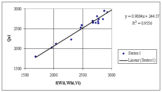
Figure 1. Dependencies of Qsi by other measured data from table 1 (see also table 2)

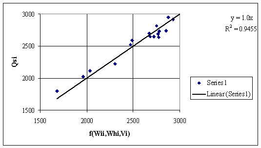
Figure 2. Dependencies of Qsi by other measured data from table 1 (see table 2 also)

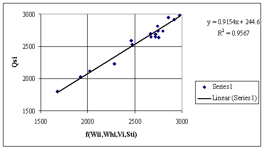
Figure 3. Dependencies of Qsi by other measured data from table 1 (see also table 2)

The fig. 3 presents the regressions between Q_si and a function that cumulate the contributions of imbibitions and hygroscopic moisture and volatile contents and also the content of total sulfur by a regular linear equation. The fig. 4 presents same dependency by an origin forced regression equation. The correlation analysis shows that total sulfur content adding do not increase de accuracy of predicted higher heating value.

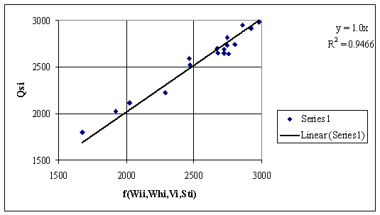
Figure 4. Dependencies of Qsi by other measured data from table 1 (see also table 2)

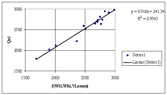
Figure 5. Dependencies of Qsi by other measured data from table 1 (see also table 2)

The fig. 5 presents the regressions between Q_si and a function that cumulate the contributions of imbibitions and hygroscopic moisture and volatile contents and also the seam identification number by a regular linear equation. The fig. 6 presents same dependency by an origin forced regression equation. The correlation analysis shows that we consider the seam number do not increase significant the accuracy of predicted higher heating value.

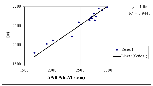
Figure 6. Dependencies of Qsi by other measured data from table 1 (see also table 2)

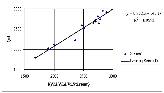
Figure 7. Dependencies of Qsi by other measured data from table 1 (see also table 2)

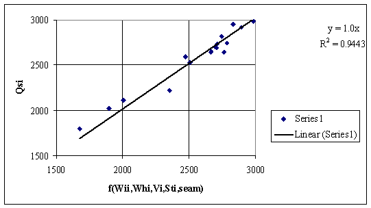
Figure 8. Dependencies of Qsi by other measured data from table 1 (see also table 2)

The fig. 7 presents the regressions between Q_si and a function that cumulate the contributions of imbibitions and hygroscopic moisture, volatile, total sulfur contents and also the seam identification number by a regular linear equation. The fig. 8 presents same dependency by an origin forced regression equation. The correlation analysis shows prove the observations from figs. 3-6, thus the best accuracy of predicted higher heating value is obtained from contributions of imbibitions and hygroscopic moisture and volatile contents.

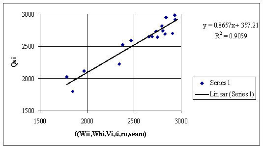
Figure 9. Dependencies of Qsi by other measured data from table 1 (see also table 2)

In the fig. 9 and 10 is presented a tries to include in higher heating value descriptor equations the ash softening temperature and the density of coal. The r value proves that the trying is uselessly.

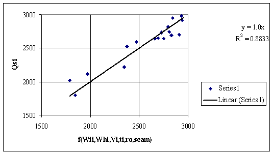
Figure 10. Dependencies of Qsi by other measured data from table 1 (see also table 2)

The dependency plotted in fig. 11 considers a function that cumulates the contributions of fixed carbon and volatile contents. Apparently, the correlation analysis does not show a better correlation than previous results. But, looking at fig. 12, where are considerate also the contribution of hygroscopic moisture content, it can observe that the predictor function is comparable in power of estimation with predictor from fig. 1.

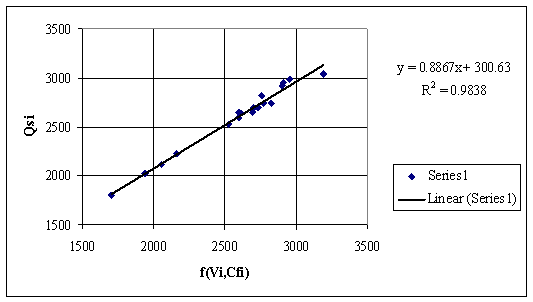
Figure 11. Dependencies of Q_si by a C_fi based equation

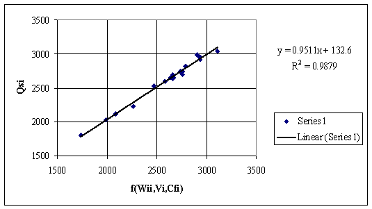
Figure 12. Dependencies of Q_si by a C_fi based equation

Another prediction tries is depicted in fig. 13, where the contributions of volatiles, fixed carbon and total sulfur are considered. The r value proves that the trying was successful, the predictor is better than previous ones.

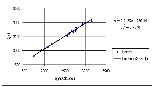
Figure 13. Dependencies of Q_si by a C_fi based equation

Last figure (fig. 14) presents also a very good correlation and is based on both fig. 1 and fig. 13 observations. The dependency includes imbibitions and hygroscopic moisture, volatile, fixed carbon and sulfur contents.

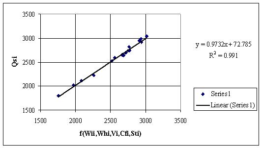
Figure 14. Dependencies of Q_si by a C_fi based equation

Conclusions

The study shows the possibility of reducing number of analysis for physical and chemical parameters of coals without reducing the quality of information. The study shows the possibility of prediction of higher heating value from another measured data. From fig. 1 it result that if are available only imbibitions and hygroscopic moisture and volatile contents is proper to predict higher heating value from them. From fig. 13 it result that if are available only fixed carbon, volatile and sulfur content, is proper to predict higher heating value from them. Finally, from fig. 14 it result that if are available imbibitions and hygroscopic moisture, volatile, fixed carbon and sulfur contents, the best choice to predict the higher heating value is to consider all of them.

References

1. http://microsoft.com

2. http://www.mozilla.org

3. http://www.opera.com

4. http://www.netscape.com

5. http://www.konqueror.org

6. H. Nascu, L. Jäntschi, T. Hodisan, C. Cimpoiu, G. Câmpan, Some Applications of Statistics in Analytical Chemistry, Reviews in Analytical Chemistry, Freud Publishing House, XVIII(6), 1999, 409-456.

7. L. Jäntschi, G. Katona, M. Diudea, Modeling Molecular Properties by Cluj Indices, Commun. Math. Comput. Chem. (MATCH), 2000, 41, 151-188, ISSN 0340-6253.

8. L. Jäntschi, H. Nascu, Numerical Description of Titration (MathCad application), International Conference on Quality Control, Automation and Robotics, May 23-25 2002, Cluj-Napoca, Romania, work published in volume "AQTR Theta 13" (ISBN 973-9357-10-3) at p. 259-262.

9. M. Diudea, L. Jäntschi, A. Graovac, Cluj Fragmental Indices, Math/Chem/Comp'98 (The Thirteenth Dubrovnik International Course & Conference on the Interfaces among Mathematics, Chemistry and Computer Sciences), June 22-27, 1998.

10. L. Jäntschi, M. Unguresan, Parallel processing of data. C++ Applications, Oradea University Annals, Mathematics Fascicle, 2001, VIII, 105-112, ISSN 1221-1265.

11. L. Jäntschi, M. Unguresan, MathLab. Statistical Applications, International Conference on Quality Control, Automation and Robotics, May 23-25 2002, Cluj-Napoca, Romania, work published in volume "AQTR Theta 13" (ISBN 973-9357-10-3) at p. 194-199.

12. L. Marta, I. G. Deac, I. Fruth, M. Zaharescu, L. Jäntschi, Superconducting Materials: Comparision Between Coprecipitation and Solid State Phase Preparation, International Conference on Science of Materials, August 20-22, 2000, Cluj-Napoca, Romania, work published in volume 2 (ISBN 973-686-058-2) at p. 627-632.

13. C. Sârbu, L. Jäntschi, Statistic Validation and Evaluation of Analytical Methods by Comparative Studies. I. Validation of Analytical Methods using Regression Analysis (in Romanian), Revista de Chimie, Bucuresti, 49(1), 1998, 19-24, ISSN 0034-7752.

14. Lorentz JÄNTSCHI, Automat Server Side Processing of Statistical Data, UNITECH'02 International Scientific Conference, November 21-22 2002, Gabrovo, Bulgaria, work published in volume "ISC UNITECH'02 GABROVO Proceedings" (ISBN 954-683-167-0) at p. 185-189.

15. Blum I., Barca Fr., Chemistry and preparation of solid combustors (in Romanian), Ed. Did. Ped., Bucharest, 1966.

16. Enache C-tin., Focşa I., Pică Elena Maria, Niac G., The Study of Lignite from the Fărcăşeşti Area, Acta Technica Napocensis, Section: Construction Machines and Materials, 36 (1993), pp.79-86.