Binomial Distribution Sample Confidence Intervals Estimation: 1. Sampling and Medical Key Parameters Calculation from Leonardo Electronic Journal of Practices and Technologies

Binomial Distribution Sample Confidence Intervals Estimation

1. Sampling and Medical Key Parameters Calculation

Tudor DRUGAN^a, Sorana BOLBOACĂ^a*, Lorentz JÄNTSCHI^b,

Andrei ACHIMAŞ CADARIU^a

^a “Iuliu Haţieganu” University of Medicine and Pharmacy, Cluj-Napoca, Romania

^b Technical University of Cluj-Napoca, Romania

* corresponding author, sbolboaca@umfcluj.ro

Abstract

The aim of the paper was to present the usefulness of the binomial distribution in studying of the contingency tables and the problems of approximation to normality of binomial distribution (the limits, advantages, and disadvantages). The classification of the medical keys parameters reported in medical literature and expressing them using the contingency table units based on their mathematical expressions restrict the discussion of the confidence intervals from 34 parameters to 9 mathematical expressions. The problem of obtaining different information starting with the computed confidence interval for a specified method, information like confidence intervals boundaries, percentages of the experimental errors, the standard deviation of the experimental errors and the deviation relative to significance level was solves through implementation in PHP programming language of original algorithms. The cases of expression, which contain two binomial variables, were separately treated. An original method of computing the confidence interval for the case of two-variable expression was proposed and implemented. The graphical representation of the expression of two binomial variables for which the variation domain of one of the variable depend on the other variable was a real problem because the most of the software used interpolation in graphical representation and the surface maps were quadratic instead of triangular. Based on an original algorithm, a module was implements in PHP in order to represent graphically the triangular surface plots. All the implementation described above was uses in computing the confidence intervals and estimating their performance for binomial distributions sample sizes and variable.

Keywords

Confidence Interval; Binomial Distribution; Contingency Table; Medical Key Parameters; PHP Applications

Introduction

The main aim of a medical research is to generate new knowledge which to be used in healthcare. Most of the medical studies generate some key parameters of interest in order to measure the effect size of a healthcare intervention. The effect size can be measure in a variety of way such as sensibility, specificity, overall accuracy and so on. Whatever the measure used are, some assessment must be made of the trustworthiness or robustness of the finding [1]. The finding of a medical study can provide a point estimation of effect and nowadays this point estimation had a confidence interval that allows us interpreting correctly the point estimation of an interest parameter.

The formal definition of a confidence interval is a confidence interval gives an estimated range of values that is likely to include an unknown population parameter, the estimated range being calculates from a given set of sample data. If independent sample are take repeatedly from same population, and a confidence interval calculated for each sample, then a certain percentage (confidence level) of the intervals will include the unknown population parameter. Confidence intervals are usually computes so that this percentage is 95%. However, we can produce 90%, 99%, 99.9% confidence intervals for an unknown parameter [2].

In medicine, we work with two types of variables: qualitative and quantitative, variables that can be classifies into theoretical distributions. Continuous variables follow a normal probability distribution, Laplace-Gauss distribution and discrete random variables follow a Binomial distribution [3].

The aim of this series of article was to review the confidence intervals used for different medical key parameters and introduce some new methods in confidence intervals estimation. The aim of the first article was to present the basic concept of confidence intervals and the problem, which can occur in confidence intervals estimation.

Binomial Distribution and its Approximation to Normality

The normal distribution was first introduced by De Moivre in an unpublished memorandum later published as part of [4] in the context of approximating certain binomial distribution for large n. His results were extends by Laplace and are now called the Theorem of De Moivre-Laplace.

Confidence interval estimations for proportions using normal approximation have been commonly uses for analysis of simulation for a simple fact: the normal approximation was easier to use in practice comparing with other approximate estimators [5].

We decided to work in our study with binomial distribution and its approximation to normality. Let’s saw how binomial distribution and its approximation to normality works! If we had from a sample size (n) a variable (X, 0 ≤ X ≤ n) which follows a binomial distribution the probability of obtaining the Y value (0 ≤ Y ≤ n) from same sample is:

(1)

The mean and the variance for the binomial variable are:

, (2)

The apparition probability of a normal variable Y (0 ≤ Y ≤ n) which has a mean M(n,X) and a standard deviation Var(n,X) is:

(3)

The approximation to normality for a binomial variable used the values of the mean and of the dispersion. Replacing the mean and the dispersion in binomial distribution formula, we obtain the next formula for 0 < X < n:

(4)

The approximation error of binomial distribution of a variable Y (0 ≤ Y ≤ n) with to normal distribution is:

(5)

Because the probability of Y decreasing with straggle of the expected value X, for mark out this digression we can adjust the expression above to zero for P_B(n,X,Y) < 1/n (in this case the differences can not be remarked for a extraction from a binomial sample):

(6)

In figure 1 was represent the approximation error of a binomial distribution with a normal distribution (using the formula above) for X/n = 1/2 where n = 10, 30, 100 and 300 (Err_c(n,n/2,Y)).

Figure 1. The approximation error of the binomial distribution with a normal distribution for X/n=1/2 where n=10, 30, 100 and 300.

If we chouse to represent the errors of the approximation of a binomial distribution with a normal distribution for X/n=1/10 where n=10, 30, 100 and 300 (Err_c(n,n/10,Y)) we obtain the below graphical representation (figure 2).

Figure 2. The approximation error of the binomial distribution with a normal distribution for X/n=1/10 where n=10, 30, 100 and 300.

The experimental errors for the 5/10 fraction (X=5, n=10) with normal approximation induce an underestimation for X = 3 and X = 7 with a sum of 7.8‰ and an overestimation for X = 4, X = 5 and X = 6 with a percent sum of 8.3‰ which compared with the choused significance level α = 5% represent less than 10%. However, the error variation shows us that the normal approximation induce a decreasing of the confidence interval for a proportion being considered more frequently the values neighbor to the 5 than the extremities values.

Graphical representation for the variation of the errors sum of positive estimation (for the values away to the measured values) and the variation of the error sum of negative estimation (for the values closed to the measured values) in logarithmical scale (n, and the errors sum) was presented in figure 3.

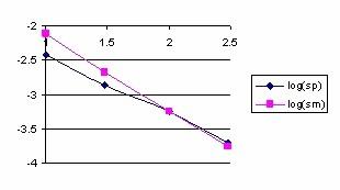
Figure 3. Logarithmical variation of the sum of positive (log(sp)) and negative(log(sm)) estimation errors depending on log(n) function for X/n = 1/2 fraction

Looking at the graphical representation from the figure 3 it can be observe that the variation of the errors sum was almost linear and inverse proportional with n. For the proportion X/n = 1/2 and generally for medium proportion the normal approximation is good and its quality increase with increasing of sample size (n). Moreover, to the surrounding of 1/2 the symmetry hypothesis of the confidence estimation induce by the normality approximation work perfectly.

Looking at the variation of the positive errors induced by the normal approximation for the proportion in form of X/n = 1/10 depending on n (see figure 4), it can be remarked that the abscissa of maximum point of deviation relative to binomial distribution are found at lower n in the vicinity of the extreme values. Thus, for n = 10, and X = 1 the error reach the maximum value of 0.108 at 0. The abscissa is moving towards X value with increasing of n (for n = 300, and X = 30 the error reach the maximum value of 0.0283 at 25).

For the variation of the negative errors induces by the normal approximation of the proportion of type X/n=1/10 depending on n, we can remark that the abscissa of maximum point of deviation depending on binomial distribution are found at lower n in the vicinity of the extreme values. Thus, for n = 10, and X = 3 the error reach the maximum value of 0.05 at 0. The abscissa is moving towards X value with increasing of n (for n = 300, and X = 30 the error reach the maximum value of 0.0260 at 34). More over, the approximation errors depending on X value is asymmetrical, and there was not any tendency for symmetry with increasing of n.

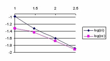
Figure 4. Logarithmic variation of the sum of values less than X (log(si)) and greater

than X (log(ss)) depending on log(n) for X/n = 1/10 fraction

Because the sum of errors for values smaller than X were always greater than the sum of errors for the values greater than X, the confidence interval obtained base don normality approximation it will be displaced to the right (there were generate more approximation errors on the left side).

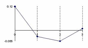
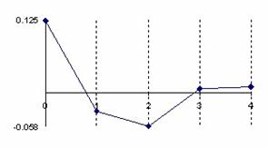
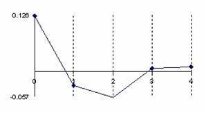
Figure 5. The error of binomial distribution approximate with a normal distribution with

X/n = 1/n fraction express through Err_c(n,1,Y) function

at n = 10, n = 30, n = 100 and n = 300

The error had a maximum value of 10.8% for n = 10 and X = 1 into point 0, value which was greater twice than the accepted significance level α = 5% (!). A maximum value of 2.6% were obtained twice consecutively for n = 30, X = 3 into the 1 and 2 points and a maximum value of 2.5% into the point 4, that was half reported to the significance level α = 5% (!); which represent a sever deviation. For large n the sum of the approximation error there was a tendency to linearity inverse proportional with n.

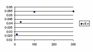
Figure 6. The variation of the error estimation sum for X/n = 1/n fraction

The graphical representations from the figure 5 and 6 reveal that for small proportions (X/n = 1/n) the sum of approximation errors were increasing with n. The sum of the approximation errors always exceeded the significance level (α = 5% (!)) for n > 50, which means that the real error threshold using normality hypothesis will exceeded 10%, the error being obtained in the favor of the greater values for the X.

Implementation of the Mathematical Calculation in MathCad

The experimental described in the previous section was possible after a MathCad implementation. The results obtained running the MathCad program were imports in Microsoft Excel were the graphical representations were creates.

In MathCad were implements the next functions:

· n combination taking to k: was necessary a logarithmical expression because we were working with large sample size and for n = 300 we could not used the classical formula C(n,k) = n!/((n-k)!k!)

(7)

(8)

(9)

· The calculation of Y/n apparition into a binomial distribution by n sample size and X/n proportion:

(10)

· The computing of the apparition of Y/n into a normal distribution sample by volume n, mean X/n and variance X(n-X)/n:

(11)

· The differences between the binomial and normal distribution:

(12)

· Initializations (needed for defining the series of values):

(values which were consecutively changed with 10,1; 10,5; 30,1; 30,3; 30,15; 100,1; 100,10; 100,50; 300,1; 300,30; 300,150)

· The computing of the series of corrected differences (graphically represented in figure 1, 2 and 5):

(13)

· The construction of the series of the positive sum of probabilities differences until to X (graphically represented in figure 3)

(14)

· The construction of the series of the positive sum of probabilities differences for the values less than X/n (graphically represented in figure 4)

(15)

- display the values of the sum for each pair of data

· The calculation of the differences probabilities for every parameters:

display the values of the sum for each pair of data (16)

Was also used a File Read/Write component (linked with dBNC_Y) in order to export the results into *.txt file from where the data were imported in Microsoft Excel where the graphical representation were drawing.

Generating a Binomial Sample using a PHP Program

In order to evaluate the confidence intervals for medical key parameters we decide to work with binomial samples and variables. In PHP was creates a module with functions that generates binomial distribution probabilities. Each by another, was implements functions for computing the binomial coefficient of n vs. k (bino0 function), the binomial probability for n, X, Y (bino1, bino2, and bino3 functions), drawing out a binomial sample of size n_es (bino4 function). Finally, array rearrangement of binomial sample values staring with position 0 and saving in the last element the value of rearrangement postponement are makes by bino5 function.

The used functions are:

function bino0($n,$k){ $rz = 1;

if($k<$n-$k) $k=$n-$k;

for ($j=1;$j<=$n-$k;$j++)

$rz *= ($k+$j)/$j;

return $rz; }

function bino1($n,$y,$x){ return pow($x/$n,$y)*pow(1-$x/$n,$n-$y)*bino0($n,$y); }

function bino2($n,$y,$x){

if(!$x) if($y) return 0; else return 1;

$nx=$n-$x; $ny=$n-$y;

if(!$nx) if($ny) return 0; else return 1;

$ret=0;

if($y){

$ret += log($x)*$y;

if($ny){

$ret += log($nx)*$ny;

if($ny>$y) $y=$ny;

for($k=$y+1;$k<=$n;$ret+=log($k++));

for($k=2;$k<=$n-$y;$ret-=log($k++)); }

} else $ret += log($nx)*$ny;

return exp($ret-log($n)*$n); }

function bino3($n,$y,$x){

if(!$x) if($y) return 0; else return 1;

$x/=$n; $nx=1-$x; $ny=$n-$y;

if(!$nx) if($ny) return 0; else return 1;

$ret=0;

if($y){

$ret += log($x)*$y;

if($ny){

$ret += log($nx)*$ny;

if($ny>$y) $y=$ny;

for($k=$y+1;$k<=$n;$ret+=log($k++));

for($k=2;$k<=$n-$y;$ret-=log($k++)); }

} else $ret += log($nx)*$ny;

return exp($ret); }

function bino4($n,$k,$n_es){

for($j=0;$j<=$n;$j++){

if($j>15) $c[$j]=bino1($n,$j,$k); else $c[$j]=bino3($n,$j,$k);

$c[$j]=round($c[$j]*$n_es);

if(!$c[$j])unset($c[$j]); }

return $c; }

function bino5($N,$k,$f_N){

$d=bino4($N,$k,$f_N);

$j=0;

foreach($d as $v) $r[$j++]=$v;

foreach($d as $i => $v) break;

$r[count($r)]=$i;

return $r; }

Computing the confidence intervals for a binomial variable is time consuming. In this perspective, an essential problem was optimizing the computing time. We studied comparative the time needed for generating the binomial probabilities using the bino1 function, the bino2 function, and the bino3 function. We developed a module which to collect and display the execution time. In the appreciation of the execution time, we used the internal clock of the computer.

The module that collects and displays the execution time is:

$af="N\tBino1\tBino2\tBino3\r\n";

for($n=$st;$n<$st+1;$n++){

$t1=microtime(TRUE);

for($x=0;$x<=$n;$x++) for($y=0;$y<=$n;$y++)

$b=bino1($n,$y,$x);

$t2=microtime(TRUE);

for($x=0;$x<=$n;$x++) for($y=0;$y<=$n;$y++)

$b=bino2($n,$y,$x);

$t3=microtime(TRUE);

for($x=0;$x<=$n;$x++) for($y=0;$y<=$n;$y++)

$b=bino3($n,$y,$x);

$t4=microtime(TRUE);

$af.=$n."\t";

$af.=sprintf("%5.3f",log((10000*($t2-$t1))))."\t";

$af.=sprintf("%5.3f",log((10000*($t3-$t2))))."\t";

$af.=sprintf("%5.3f",log((10000*($t4-$t3))))."\r\n";}

echo($af);

Table 1 contains the logarithmical values of the executions time for n: 3, 10, 30, 50, 100, 150, and 300 obtained by the bino1, bino2, and bino3 functions.

n	Bino1	Bino2	Bino3
3	1.92	1.573	1.406
10	3.975	4.021	3.956
30	6.441	6.763	6.74
50	7.731	8.149	8.137
100	9.576	10.108	10.101
150	10.706	11.28	11.278
300	12.691	13.314	13.314

Table 1. The execution time (seconds) express in logarithmical scale needed for generating binomial probabilities with implemented function

The differences between executions time express in logarithmical scale for the functions bino1and bino3 and respectively for the functions bino2 and bino3 were uses in order to obtain the graphical representations from the figure 3. Looking at the execution time ratio for the bino1 and bino3 function (the Bino2-Bino3 curve, figure 3) we can remark that optimizing parameter with X/n instead of X and (n-X)/n instead of (n-X) bring an increasing performance; this increased performance was cancel with increasing of n (the logarithmical difference was almost 0 for n >50).

Looking at the execution time ratio for the bino2 and bino3 functions (the Bino2-Bino3 curve, figure 3) we can remark that with increasing of n the bino3 function obtained the best performance comparing with bino1 and bino2 (the differences between execution time express in logarithmical scale became less than 0 beginning with n ≈ 15). Based on above observations, was implements for the binomial probabilities estimation the bino4 function.

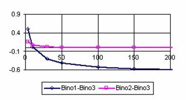
Figure 3. Binomial probabilities execution time for bino1, bino2, and bino3 functions

Medical Key Parameters on 2´2 Contingency Table

For the 2´2 contingency table data and based on the type of the medical studies we can compute some key parameters used for interpreting the studies results. Let us suppose that we have a contingency table as the one in the table 2.

		Result/Disease (Characteristic B)
		Positive	Negative	Total
Treatment / Risk factor / Diagnostic Test (Characteristic A)	Positive	a	b	a+b
	Negative	c	d	c+d
	Total	a+c	b+d	a+b+c+d

Table 2. Hypothetical 2´2 contingency table

In table 2, a denotes the real positive cases (those who have both characteristics), b the false positive cases (those who have just the characteristic A), c the false negative cases (those who have the characteristic B) and d the real negative cases (those who have neither characteristic).

We classified the medical key parameters based on the mathematical expressions (see table 3). This classification was very useful in confidence intervals assessment for each function, and for implementing the function in PHP.

The PHP functions for the mathematical expression described in the table 3 had the next expressions:

function ci1($X,$n){

return $X/$n; }

function ci2($X,$n){

if($X==$n) return (float)"INF";

return $X/($n-$X); }

function ci3($X,$n){

if(2*$X==$n) return (float)"INF";

return $X/(2*$X-$n); }

function ci4($X,$m,$Y,$n){

if(($X==$m)||($Y==0)) return (float)"INF";

return $X*($n-$Y)/$Y/($m-$X); }

function ci5($X,$m,$Y,$n){

return $Y/$n-$X/$m; }

function ci6($X,$m,$Y,$n){

return abs(ci5($X,$m,$Y,$n)); }

function ci7($X,$m,$Y,$n){

$val=ci6($X,$m,$Y,$n);

if(!$val) return (float)"INF";

return 1/$val; }

function ci8($X,$m,$Y,$n){

if($Y==0) return (float)"INF";

return ci1($X,$m)/ci1($Y,$n); }

function ci9($X,$m,$Y,$n){

if($Y==0) return (float)"INF";

return abs(1-ci1($X,$m)/ci1($Y,$n)); }

No	Mathematical expression and PHP function	Name of the key parameter	Type of study
1	, ci1	Individual Risk on Exposure Group and NonExposure Group	Risk factor or prognostic factor studies [6], [7]
		Experimental and Control Event Rates Absolute Risk in Treatment and Control Group	Therapy studies [8], [9]
		Sensitivity; Specificity; Positive and Negative Predictive Value; False Positive and Negative Rate; Probability of Disease, Positive and Negative Test Wrong; Overall Accuracy; Probability of a Negative and Positive Test	Diagnostic studies [10], [11], [12]
2	, ci2	Post and Pre Test Odds	Diagnostic studies 7, 9, 10]
3	, ci3	Post Test Probability	Diagnostic studies [9, 10]
4	, ci4	Odds Ratio	Risk Factor studies [6, 7]
5	, ci5	Excess risk	Risk Factor studies [5]
6	, ci6	Absolute Risk Reduction and Increase, Benefit Increase	Therapy studies 7, 9]
7	, ci7	Number Needed to Treat and Harm	Therapy studies [7, 9]
8	, ci8	Relative Risk	Studies of Risk Factor [5, 6]
8	, ci8	Positive and Negative Likelihood Ratio	Diagnostic studies [7, 9, 10]
9	, ci9	Relative Risk Reduction, Increase and Benefit Increase	Therapy studies [7, 9]

Table 3. Mathematical expressions and PHP functions for medical key parameters

Estimating Confidence Intervals using a PHP program

In order to be able to check out if that the experimental numbers belong to confidence interval were implements in PHP two functions, one named out_ci_X for one-variable functions (depending on X) and the other, named out_ci_XY for two-variables functions (depending on X, Y). The functions had the expressions:

function out_ci_X(&$cif,$XX,$X,$n,$z,$a,$f,$g){

$ci_v=ci($cif,$g,$X,$n,$z,$a);

if(!is_finite($ci_v[1])) return 0;

if(!is_finite($ci_v[0])) return 0;

$ci_v=ci($cif,$g,$XX,$n,$z,$a);

if(!is_finite($ci_v[1])) return 0;

if(!is_finite($ci_v[0])) return 0;

$fx=$f($X,$n);

if(!is_finite($fx)) return 0;

return (($fx<$ci_v[0])||($fx>$ci_v[1]));}

function out_ci_XY(&$cif,$XX,$X,$YY,$Y,$m,$n,$z,$a,$f){

$ci_v=$cif($XX,$m,$YY,$n,$z,$a);

if(!is_finite($ci_v[0])) return 0;

if(!is_finite($ci_v[1])) return 0;

$fxy=$f($X,$m,$Y,$n);

if(!is_finite($fxy)) return 0;

return (($fxy<$ci_v[0])||($fxy>$ci_v[1]));}

The function est_ci_er compute the confidence interval boundaries, the experimental errors, the mean, and the standard deviation for the expression with one variable (X); the est_ci2_er was the function for the two-variable expressions (X, Y):

function est_ci_er($z,$a,$c_i,$g,$f,$ce){

if($ce=="ci") est_X(z,a,$c_i,$f,$g);

if($ce=="er") est_N(z,a,$c_i,$f,$g,1);

if($ce=="me") est_N(z,a,$c_i,$f,$g,2);

if($ce=="va") est_N(z,a,$c_i,$f,$g,3);

if($ce=="mv") est_N(z,a,$c_i,$f,$g,6);}

function est_ci2_er($z,$a,$c_i,$f,$ce){

if($ce=="ci") est_X2(z,a,$c_i,$f);

if($ce=="er") est_N2(z,a,$c_i,$f);

if($ce=="me") est_MN(z,a,$c_i,$f,2);

if($ce=="va") est_MN(z,a,$c_i,$f,3);

if($ce=="mv") est_MN(z,a,$c_i,$f,6);}

The est_X compute all the confidence intervals for the one-variable functions (depending on X) while est_X2 compute the confidence intervals for two-variable functions (depending on X, Y):

function est_X($z,$a,$c_i,$f,$g){

echo("N\tX\tf(X)");

for($i=0;$i<count($c_i);$i++){

echo("\t".$c_i[$i]."L");

echo("\t".$c_i[$i]."U"); }

for($n=N_min;$n<N_max;$n++){

for($X=0;$X<=$n;$X++){

for($i=0;$i<count($c_i);$i++)

$ci[$i] = ci($c_i[$i],$g,$X,$n,$z,$a);

$fX = $f($X,$n);

echo("\r\n".$n."\t".$X."\t".trim(sprintf("%6.3f",$fX)));

for($k=0;$k<count($c_i);$k++){

echo("\t".trim(sprintf("%6.3f",$ci[$k][0])));

echo("\t".trim(sprintf("%6.3f",$ci[$k][1]))); } }}}

function est_X2($z,$a,$c_i,$f){

echo("X\tY\tf(X,Y)");

for($i=0;$i<count($c_i);$i++){

echo("\t".$c_i[$i]."L");

echo("\t".$c_i[$i]."U"); }

for($n=N_min;$n<N_max;$n++){

$m = $n;

for($X=0;$X<=$m;$X++){

for($Y=0;$Y<=$n;$Y++){

for($i=0;$i<count($c_i);$i++){

$g = $c_i[$i];

$ci[$i] = $g($X,$m,$Y,$n,$z,$a); }

$fXY = $f($X,$m,$Y,$n);

echo("\r\n".$X."\t".$Y."\t".trim(sprintf("%6.3f",$fXY)));

for($k=0;$k<count($c_i);$k++){

echo("\t".trim(sprintf("%6.3f",$ci[$k][0])));

echo("\t".trim(sprintf("%6.3f",$ci[$k][1]))); } } } }}

The est_N function computed the estimation errors or means or/and standard deviations of the mean for the one-variable functions (depending on X); the est_N2 function computed the estimation errors for two-variable functions (depending on X, Y):

function est_N($z,$a,&$c_i,$cif,$g,$ce){

if($ce==1)echo("N\tX\tf(x)");else echo("N");

for($i=0;$i<count($c_i);$i++)

echo("\t".$c_i[$i]);

for($n=N_min;$n<N_max;$n++){

for($X=1;$X<p*$n;$X++){

$d=bino4($n,$X,10000);

if($ce==1) echo("\r\n".$n."\t".$X."\t".trim(sprintf("%6.3f",$cif($X,$n))));

for($i=0;$i<count($c_i);$i++){//pt fiecare ci

$ttt[$X][$i]=0;//esecuri

$conv=0;

foreach ($d as $XX => $nXX){//pt fiecare valoare posibila de esantion

if(out_ci_X($c_i[$i],$XX,$X,$n,$z,$a,$cif,$g)) $ttt[$X][$i] += $nXX;

$conv += $nXX; }

$ttt[$X][$i] *= 100/$conv;

if($ce==1)echo("\t".trim(sprintf("%3.3f",$ttt[$X][$i]))); } }

if ($ce > 1) est_MV($ttt,count($c_i),$n,p,0,$ce,$a); }}

function est_N2($z,$a,&$c_i,$f){

echo("X\tY\tf(X,Y)");

for($i=0;$i<count($c_i);$i++)

echo("\t".$c_i[$i]);

for($n=N_min;$n<N_max;$n++){

$m = $n;

for($X=1;$X<p*$m;$X++){

$dX=bino4($m,$X,1000);

for($Y=1;$Y<p*$n;$Y++){

$dY=bino4($n,$Y,1000);

echo("\r\n".$X."\t".$Y."\t".trim(sprintf("%3.3f",$f($X,$m,$Y,$n))));

for($i=0;$i<count($c_i);$i++){

$ttt[$X][$Y][$i]=0;//esecuri

$conv=0;

foreach ($dX as $XX => $nXX){

foreach ($dY as $YY => $nYY){

if(out_ci_XY($c_i[$i],$XX,$X,$YY,$Y,$m,$n,$z,$a,$f))

$ttt[$X][$Y][$i] += $nXX*$nYY;

$conv += $nXX*$nYY; } }

echo("\t".trim(sprintf("%3.3f",100*$ttt[$X][$Y][$i]/$conv))); } } } }}

The est_MN function computed the means and/or the standard deviations of the mean for the two-variable functions (depending on X, Y):

function est_MN($z,$a,&$c_i,$f,$ce){

echo("M\tN");

for($i=0;$i<count($c_i);$i++)

echo("\t".$c_i[$i]);

for($m=N_min;$m<N_max;$m++){

for($n=N_min;$n<N_max;$n++){

for($i=0;$i<count($c_i);$i++){

if($ce % 2 == 0) $md[$i] = 0;

if($ce % 3 == 0) $va[$i] = 0; }

for($X=1;$X<p*$m;$X++){

$dX=bino4($m,$X,10000);

for($Y=1;$Y<p*$n;$Y++){

$dY=bino4($n,$Y,10000);

for($i=0;$i<count($c_i);$i++){

$ttt[$X][$Y][$i]=0;//esecuri

$conv=0;

foreach ($dX as $XX => $nXX){

foreach ($dY as $YY => $nYY){

if(out_ci_XY($c_i[$i],$XX,$X,$YY,$Y,$m,$n,$z,$a,$f))

$ttt[$X][$Y][$i] += $nXX*$nYY;

$conv += $nXX*$nYY; } }

if($ce % 2 == 0) $md[$i] += 100*$ttt[$X][$Y][$i]/$conv;

if($ce % 3 == 0) $va[$i] += pow(100*$ttt[$X][$Y][$i]/$conv-5,2); } } }

echo("\r\n".$m."\t".$n);

for($i=0;$i<count($c_i);$i++){

if($ce % 2 == 0)

echo("\t".trim(sprintf("%3.3f",$md[$i]/($m-1)/($n-1))));

if($ce % 3 == 0)

echo("\t".trim(sprintf("%3.3f",sqrt($va[$i]/(($m-1)*($n-1)-1))))); } } }}

The est_MV function computed the estimation errors means and/or standard deviations:

function est_MV(&$ttt,$n_c_i,$n,$p,$v,$ce,$a){

for($i=0;$i<$n_c_i;$i++){

$md[$i]=$v; if($v)continue;

if($p==0.5){

for($X=1;$X<$p*$n;$X++) $md[$i]+=2*$ttt[$X][$i];

if(is_int($p*$n)) $md[$i]+=$ttt[$p*$n][$i];

$md[$i]/=($n-1);

} else {

for($X=1;$X<$p*$n;$X++) $md[$i]+=$ttt[$X][$i];

$md[$i]/=($n-1); } }

if($ce % 3 == 0)

for($i=0;$i<$n_c_i;$i++){

$ds[$i]=0;

if($p==0.5){

for($X=1;$X<$p*$n;$X++){

$ds[$i]+=2*pow($ttt[$X][$i]-$md[$i],2); }

if(is_int($p*$n)) $ds[$i]+=pow($ttt[$X][$i]-100*$a,2);//$md[$i],2);

$ds[$i]/=($n-2);//s

$ds[$i]=pow($ds[$i],0.5);

} else {

for($X=1;$X<$p*$n;$X++){

$ds[$i]+=pow($ttt[$X][$i]-100*$a,2);//$md[$i],2); }

$ds[$i]/=($n-2);//s

$ds[$i]=pow($ds[$i],0.5); } }

if($ce % 2 == 0){

echo("\r\n".$n);

for($i=0;$i<$n_c_i;$i++)

echo("\t".trim(sprintf("%3.3f",$md[$i]))); }

if($ce % 3 == 0){

echo("\r\n".$n);

for($i=0;$i<$n_c_i;$i++)

echo("\t".trim(sprintf("%3.3f",$ds[$i]))); }}

The est_R2 function compute and display, for a 100 random sample size and binomial variables values the experimental errors using the imposed (theoretical) value of significance level for all confidence interval calculation methods given also as parameter:

function est_R2($z,$a,&$c_i,$f){

echo("p\tM\tN\tX\tY\tf(X,Y)");

for($i=0;$i<count($c_i);$i++)

echo("\t".$c_i[$i]);

for($k=0;$k<100;$k++){

$n = rand(4,1000);

$m = rand(4,1000);

$X = rand(1,$m-1);

$Y = rand(1,$n-1);

$dX=bino4($m,$X,10000);

$dY=bino4($n,$Y,10000);

echo("\r\n".$k."\t".$m."\t".$n."\t".$X."\t".$Y."\t".trim(sprintf("%3.3f",$f($X,$m,$Y,$n))));

for($i=0;$i<count($c_i);$i++){//pt fiecare ci

$ttt[$X][$Y][$i]=0;//esecuri

$conv=0;

foreach ($dX as $XX => $nXX){

foreach ($dY as $YY => $nYY){

if(out_ci_XY($c_i[$i],$XX,$X,$YY,$Y,$m,$n,$z,$a,$f))

$ttt[$X][$Y][$i] += $nXX*$nYY;

$conv += $nXX*$nYY;

}

echo("\t".trim(sprintf("%3.3f",100*$ttt[$X][$Y][$i]/$conv)));

}

The est_C2 function compute and display for a fixed value of proportion X/n (usually the central point X/n = 1/2) the errors for a series of sample size (from N_min to N_max):

function est_C2($z,$a,&$c_i,$f){

echo("X\tY\tf(X,Y)");

for($i=0;$i<count($c_i);$i++)

echo("\t".$c_i[$i]);

for($n=N_min;$n<N_max;$n+=4){

$m = $n;

//$X = (int)(3*$m/4); $Y = (int)($n/4);

$X = (int)($m/2); $Y = (int)($n/2);

$dX=bino4($m,$X,10000);

//$dY=bino4($n,$Y,10000);

$dY=$dX;

echo("\r\n".$X."\t".$Y."\t".trim(sprintf("%3.3f",$f($X,$m,$Y,$n))));

for($i=0;$i<count($c_i);$i++){

$ttt[$X][$Y][$i]=0;//esecuri

$conv=0;

foreach ($dX as $XX => $nXX){

foreach ($dY as $YY => $nYY){

if(out_ci_XY($c_i[$i],$XX,$X,$YY,$Y,$m,$n,$z,$a,$f))

$ttt[$X][$Y][$i] += $nXX*$nYY;

$conv += $nXX*$nYY;

}

echo("\t".trim(sprintf("%3.3f",100*$ttt[$X][$Y][$i]/$conv)));

}

The ci function used in est_N, est_N2, est_X, and est_X2 functions compute the confidence interval for specified function with specified parameter and it was uses for the nine functions described in table 3. Corresponding to the functions described in table 3, were defines:

· the I function for the expression X/n;

· the R function was used for the expression X/(n-X);

· the RD function was used for the expression X/(2X-n);

· the R2 function for the expression X(n-Y)/Y/(m-X);

· the D function for the expression Y/n-X/n;

· the AD function for the expression |Y/n-X/n|;

· the IAD function for the expression 1/|Y/n-X/n|;

· the RP function for the expression Xn/Y/m;

· the ARP function for the expression |1- Xn/Y/m|.

For the one-variable expressions (f(X)) the confidence intervals was compute using the next expressions:

· For ci1 function:

o Mathematical expression: (17)

where CI_L(X) and CI_U(X) were the lower limit and respectively the upper limit of the confidence interval;

o PHP function:

function I($f,$X,$n,$z,$a){

return $f($X,$n,$z,$a);}

· For ci2 function:

o Mathematical expression: (18)

o PHP function:

function R($f,$X,$n,$z,$a){

$L = $f($X,$n,$z,$a);

if ($L[1])

if ($L[1]-1) $Xs = 1/(1/$L[1]-1); else $Xs = (float) "INF";

else $Xs = 0;

if ($L[0]-1)

if ($L[0]) $Xi = 1/(1/$L[0]-1); else $Xi = 0;

else $Xi = 0;

return array ( $Xi , $Xs );}

· For ci3 function; the expression for confidence interval is based on confidence intervals expression used for ci1:

o Mathematical expression: (19)

o PHP function:

function RD($f,$X,$n,$z,$a){

if($X==$n-$X) return array( -(float)"INF" , (float)"INF" );

$q=$f($X,$n,$z,$a);

if($X==$n) return array ( 1/$q[1] , 1/$q[0] );

if($q[0]==0) $tXs = 0; else $tXs = 1/(2-1/$q[0]);

if($q[1]==0.5)

$tXi=-(float)"INF";

else if(!$q[1])

$tXi=0;

else

$tXi = 1/(2-1/$q[1]);

if($X){

$tX= 1/(2-$n/$X);

if(($tXi>$tX)||($tXs<$tX)) {

$tnX=1/(2-$n/($n-$X));

if(abs($tnX)<abs($tX))$tX=$tnX;

$tXi = $tX * exp(exp(abs($tX)));

$tXs = -$tX * exp(exp(abs($tX))); } }

return array( $tXi , $tXs );}

The formulas for computing the confidence intervals for two-variable functions (depending on X, Y) can be express base on the formulas for confidence intervals of one-variable functions (depending on X):

· For ci4 function:

o Mathematical expression: (20)

o PHP function:

function R2($f,$X,$m,$Y,$n,$z,$am,$an){

$ciX = R($f,$X,$m,$z,$am);

$cinY = R($f,$n-$Y,$n,$z,$an);

return array ( $ciX[0]*$cinY[0] , $ciX[1]*$cinY[1] );}

· For ci5 function:

o Mathematical expression: (21)

o PHP function:

function D($f,$X,$m,$Y,$n,$z,$am,$an){

$ciX = $f($X,$m,$z,$am);

$ciY = $f($Y,$n,$z,$an);

return array ( $ciY[0]-$ciX[1] , $ciY[1]-$ciX[0] );}

· For ci6 function:

o Mathematical expression:

(22)

o PHP function:

function AD($ci){

if($ci[0]*$ci[1]<=0){

$max =abs($ci[0]);

if($max<abs($ci[1])) $max = abs($ci[1]);

return array ( 0 , $max );

}else{

if($ci[0]<0) {

$ci[0] = abs($ci[0]);

$ci[1] = abs($ci[1]); }

if($ci[0]<$ci[1]) return array( $ci[0] , $ci[1] );

else return array( $ci[1] , $ci[0] ); }}

· For ci7 function:

o Mathematical expression: (23)

o PHP function:

function IAD($CI){

if($CI[0]) $Xs = 1/$CI[0]; else $Xs = (float)"INF";

if($CI[0]) $Xi = 1/$CI[1]; else $Xi = (float)"INF";

return array( $Xi , $Xs );}

· For ci8 function:

o Mathematical expression: (24)

o PHP function:

function RP($f,$X,$m,$Y,$n,$z,$am,$an){

$ciX = $f($X,$m,$z,$am);

$ciY = $f($Y,$n,$z,$an);

$XYi = $ciX[0]/$ciY[1];

if($ciY[0]) $XYs = $ciX[1]/$ciY[0]; else $XYs = (float)"INF";

return array ( abs($XYi), $XYs );}

· For ci9 function:

o Mathematical expression:

o PHP function:

function ARP($f,$X,$m,$Y,$n,$z,$a){

$ci = $f($X,$m,$Y,$n,$z,$a);

if(!is_finite($ci[1])) return array ( abs(1-$ci[0]) , (float)"INF" );

$t1 = 1-$ci[0];

$t2 = 1-$ci[1];

if($t1*$t2<=0){

$Xi = 0;

if(abs($t2)>abs($t1))

return array( 0 , abs($t2) );

else

return array( 0 , abs($t1) );

}else{

if(abs($t2)>abs($t1))

return array ( abs($t1) , abs($t2) );

else

return array ( abs($t2) , abs($t1) ); }}

Were defined the normal distribution percentile (z), the error of the first kind or the significance level (a), the value for the maximum proportion for which the confidence intervals was estimated (p), the sample sizes start value (N_min) and the sample sizes stop value (N_max):

define("z",1.96);

define("a",0.05);

define("p",1);

define("N_min",10);

define("N_max",11);

A specific PHP program calls all these functions for a given n and display the estimation errors or confidence intervals limits at a specified significance level (α =5%) using est_ci_er or est_ci2_er functions. For example, in order to compute the confidence interval for a proportion (ci1 function) was call the est_ci_er function with the next parameters:

est_ci_er(z,a,$c_i,"I","ci1","ci");

where $c_i was a matrix that memorize the name of the methods used in confidence intervals estimation and I was the name of the function defined above for the expression X/n.

In the next articles, we will debate the confidence intervals methods for each function described in table 1 and their variability with sample size.

The standard deviation of the experimental error was computes using the next formula:

(26)

where StdDev(X) is standard deviation, X_i is the experimental errors for a given i (0 ≤ i ≤ n), M(X) is the arithmetic mean of the experimental errors and n is the sample size.

If we have a sample of n-1 elements (withdrawing the limits 0 and n from the 0..n array) with a known (or expected) mean ExpM(X), the deviation around α = 5% (imposed significance level) is giving by:

(27)

The (27) formula was used as a quantitative measure of deviation of errors relative to imposed error value (equal with 100α) when ExpM(X) = 100α.

Two-dimensional Functions

We used the uni-dimensional (X, m) confidence intervals functions to compute the confidence intervals for bi-dimensional functions (X, m, Y, n) but were necessary to perform a probability correction. We consider that the confidence intervals boundaries of bi-dimensional functions were gives by the product of the limits from the uni-dimensional cases with a correction of the significance level based on error convolution product.

Experimentally was infers that the best expression for the significance level for bi-dimensional function was:

or, with correction by m, (26)

where a was the uni-dimensional significance level and a_U şi a_U(m) were imposed significance level for uni-dimensional variable (X) with a volume m. Analogue can be obtained the expression for the uni-dimensional variable (Y) with a volume n, a_U(n).

Random Sampling

We consider 100 random values for n and respectively for m in the 4..1000 domain and X, respectively Y in domain 1..m-1, respectively 1..n-1. The error estimation of the confidence interval was performs for these samples and the results were graphically represented using MathCad program. Thus, we implement a module in MathCad that allowed us to perform these representations using:

· The frequencies of experimental errors;

· Dispersion relative to the imposed error value (α = 5%);

· The mean and standard deviation of the experimental errors;

· The theoretical errors distribution graphic based on Gauss distribution of means equal with five (significance level α = 5%) and standard deviation equal with a standard deviation of a volume sample size equal width 10 (double of α).

The corresponding equations are:

· (27)

· (28)

· (29)

· (30)

· (31)

· (32)

· (33)

· (34)

· (35)

· (36)

· (37)

· (38)

· (39)

· (40)

· (41)

· (42)

Graphical Representations

We developed a graphical module in PHP for graphical error map representations for bi-dimensional functions (X, m). The module used the confidence intervals computed by the program described above and performs (m, X, Z) graphical representations, where Z can be the value of the confidence intervals or the estimation errors (percentages) and perform a triangular graphical representation for Z (X on the horizontal axis; m on the vertical axis, descending order) using a color gradient. The module lines were:

define("pct",3);

define("fmin",0);

define("fmax",10);

define("ncol",21);

define("tip",1);

$file="BayesF";

g_d($file,$v);

i_p($file,$v);

function i_p(&$file,&$v){

$in=pct*($v[count($v)-1][0]+1);

$image = @imagecreate($in, $in);

$alb = imagecolorallocate($image,255,255,255);

$negru = imagecolorallocate($image,0,0,0);

$t_l = $in-imagefontwidth(2)*strlen($file)-10;

imagestring($image, 2, $t_l,10, $file, $negru);

$cl = s_c_t($image,tip);

for($k=0;$k<count($v);$k++)

for($i=0;$i<pct;$i++){

for($j=0;$j<pct;$j++){

imagesetpixel($image,pct*$v[$k][1]+$i,pct*$v[$k][0]+$j,$cl[c($v[$k][2])]); } }

imagepng($image);

//imagegif($image);

//imageinterlace($image,1);imagejpeg($image); }

function c($z){

if($z<=fmin) return 1;

if($z>=fmax) return ncol-1;

$cu = ($z-fmin)*(ncol-3)/(fmax-fmin);

$cu = (int)$cu;

return $cu + 1;}

function g_d($file,&$v){

$data=file_get_contents($file.".txt");

$r=explode("\r\n",$data);

for($i=0;$i<count($r);$i++) $v[$i]=explode("\t",$r[$i]);}

function s_c_t(&$image,$tip){

if($tip==0){//negru-alb

for ($i=0;$i<ncol;$i++){

$cb=round($i * 255/(ncol-1));

$tc[$i]=array( $cb , $cb , $cb ); } }

if($tip==1){//rosu-albastru

$tc[0] = array( 255 , 0 , 0 );

$yl = (ncol-1)/2; $yl = (int) $yl;

if($yl>1)

for($i=1;$i<$yl;$i++){

$cb = round($i * 255/$yl);

$tc[$i] = array( 255 , $cb , 0 ); }

$tc[$yl] = array( 255 , 255 , 0 );

if($yl>1)

for($i=1;$i<$yl;$i++){

$cb = round($i * 255/$yl);

$tc[$yl+$i] = array( 255-$cb , 255-$cb , $cb ); }

$tc[ncol-1] = array( 0 , 0 , 255 ); }

if($tip==2){//rosu-verde

$tc[0] = array( 255 , 0 , 0 );

$yl = (ncol-1)/2; $yl = (int) $yl;

if($yl>1)

for($i=1;$i<$yl;$i++){

$cb = round($i * 255/$yl);

$tc[$i] = array( 255 , $cb , 0 ); }

$tc[$yl] = array( 255 , 255 , 0 );

if($yl>1)

for($i=1;$i<$yl;$i++){

$cb = round($i * 255/$yl);

$tc[$yl+$i] = array( 255-$cb , 255 , 0 ); }

$tc[ncol-1] = array( 0 , 255 , 0 ); }

for ($k=0;$k<ncol;$k++)

$cl[$k]=imagecolorallocate($image,$tc[$k][0],$tc[$k][1],$tc[$k][2]);

return $cl;}

The module describe above used the pct (= 3) constant in order to represent a 3×3 pixeli square for each m, X, color(Z). The constant fmin was used to represent the values between the lower limit color (red color in our representations) and the middle limit color (yellow in our representations); the fmax constant was used to represent the maximum values which color were between upper limit color (blue) and middle limit color (yellow). All the values which not belong to the fmin , fmax] domain were represented with the lower limit color (if Z < fmin) or upper limit color (if Z > fmax). The number of shade (including the based color represented by red, yellow and blue) were defined by n_col constant (was chosen 21). The tip constant (was choose 1) define the couplet of the limit color and the corresponding shade using 3 couplet sets defined as follows: (White, Gray, Black), (Red, Yellow, Blue), and (Red, Yellow, Green).

Discussions

The approximation to normality of a binomial distribution had major disadvantages more obvious to the extremities of the proportion (X/n → 0 and X/n → 1).

Comparing different probability distribution functions revealed significant differences performances with increasing of n. The best performance methods were the functions that apply first direct and then inverse the logarithmical expression of the binomial probability function. Defining the key parameters as mathematical functions depending on random variable and sample size restrict the number of inquisition of theirs confidence intervals (from 34 medical key parameters to 9 distinct mathematical expression) (see table 3).

Working with PHP programming language offer a maximum flexibility in:

· defining and using the medical key parameters;

· defining and generating the binomial samples;

· performing the experimental of computing the confidence intervals limits;

· computing the experimental errors for each defined confidence interval methods.

For the medical key parameters, the confidence intervals expression of the parameters which depend on two random variable (X, Y) and two sample sizes (m, n) can be express based on the confidence intervals expressions for a proportion with changing the imposed value of probability.

MathCad program proved very useful in the situation were was necessary to perform complex integrals and to represent graphically the results, how was the case of the integrals based on expressions of the Gaussian function (f(x)=a∙exp((x-b)²/c²) [13]).

The tree dimensional graphical representations of the functions with two parameters (most of the medical key parameters), where the expression of the confidence intervals function of f(X,m), need a triangular grid (0 ≤ X ≤ n, were n vary on a specified domain - 4..103). There are a few software which to allow to represent correctly these kind of triangular plots, most of the software used some interpolation functions and the graphical representation are square plots (0 ≤ X ≤ 103; 4 ≤ n ≤ 103) instead of triangular plots (0 ≤ X ≤ n; 4 ≤ n ≤ 103). Thus was necessary to used PHP in order to create correct error maps.

All the aspects presented in this paper uses in the confidence intervals estimations for the key parameters used as measure the effect size for different healthcare intervention express as different medical key parameters (see further papers).

References