Binomial Distribution Sample Confidence Intervals Estimation
2. Proportion-like Medical Key Parameters
Sorana BOLBOACĂ*, Andrei ACHIMAŞ CADARIU
Iuliu Haţieganu University of Medicine and Pharmacy, Cluj-Napoca, Romania
* corresponding author, sbolboaca@umfcluj.ro
Abstract
The accuracy of confidence interval expressing is one of most important problems in medical statistics. In the paper was considers for accuracy analysis from literature, a number of confidence interval formulas for binomial proportions from the most used ones.
For each method, based on theirs formulas, were implements in PHP an algorithm of computing.
The performance of each method for different sample sizes and different values of binomial variable was compares using a set of criteria: the average of experimental errors, the standard deviation of errors, and the deviation relative to imposed significance level. A new method, named Binomial, based on Bayes and Jeffreys methods, was defines, implements, and tested.
The results show that there is no method from considered ones, which to have a constant behavior in terms of average of the experimental errors, the standard deviation of errors, or the deviation relative to imposed significance level for every sample sizes, binomial variables, or proportions of them. More, this unfortunately behavior remains also for large and small subsets of natural numbers set. The Binomial method obtained systematically lowest deviations relative to imposed significance level (α = 5%) starting with a certain sample size.
Keywords
Confidence Intervals; Binomial Proportion; Proportion-like Medical Parameters
Introduction
In the medical studies, many parameters of interest are compute in order to assess the effect size of healthcare interventions based on 2´2 contingency table and categorical variables. If we look for example at diagnostic studies, we have the next parameters that can be express as a proportion: sensitivity, specificity, positive predictive value, negative predictive value, false negative rate, false positive rate, probability of disease, probability of positive test wrong, probability of negative test wrong, overall accuracy, probability of a negative test, probability of a positive test [1], [2], [3]. For the therapy studies experimental event rate, control event rate, absolute risk in treatment group, and absolute risk on control group are the proportion-like parameter [4], [5] which can be compute based on 2´2 contingency table. If we look at the risk factor studies, the individual risk on exposure group and individual risk on nonexposure group are the parameters of interest because they are also proportions [6]. Whatever the measure used, some assessment must be made of the trustworthiness or robustness of the findings, even if we talk about a p-value or confidence intervals. The confidences intervals are preferred in presenting of medical results because are relative close to the data, being on the same scale of measurements, while the p-values is a probabilistic abstraction [7]. Rothmans sustained that confidence intervals convey information about magnitude and precision of effect simultaneously, keeping these aspects of measurement closely linked [8]. The confidence intervals estimation for a binomial proportion is a subject debate in many scientific articles even if we talk about the standard methods or about non asymptotic methods [9], [10], [11], [12]. It is also known that the coverage probabilities of the standard interval can be erratically poor even if p is not near the boundaries 10, [13], [14], [15]. Some authors recommend that for the small sample size n (40 or less) to use the Wilson or the Jeffreys confidence intervals method and for the large sample size n (> 40) the Agresti-Coull confidence intervals method [10].
The aim of this research was to assess the performance for a binomial distribution samples of literature reported confidence intervals formulas using a set of criterions and to define, implement, and test the performance of a new original method, called Binomial.
Materials and Methods
In literature, we found some studies that present the confidence intervals estimation for a proportion based on normal probability distribution or on binomial probability distribution, or an binomial distribution and its approximation to normality [16].
In this study, we compared some confidence intervals expressions, which used the hypothesis of normal probability distribution, and some confidence intervals formula, which used the hypothesis of binomial probability distribution. It is necessary to remark that the assessment of the confidence intervals, which used the hypothesis of binomial distribution, is time-consuming comparing with the methods, which used the hypothesis of a normal distribution.
In order to assess, both confidence intervals estimation aspects, quantitative and qualitative, and the performance of a confidence interval comparative with other methods we developed a module in PHP. The module was able to compute and evaluate the confidence intervals for a given X and a given n, build up a binomial distribution sample (XX) based on given X and compute the experimental errors of X values into its confidence intervals of xxÎXX for each specified methods. We choose in our experiments a significance level equal with α = 5% (α = 0.05; noted a in our program) and the corresponding normal distribution percentile z1-α/2 = 1.96 (noted z in the program) for the confidence intervals which used normal distribution probability. The value of sample size (n) was chosen in the conformity with the real number from the medical studies; in our experiments, we used 4 ≤ n ≤ 1000. The estimation of the errors were performed for the value of X variable which respect the rule 0 < X < n. The confidence intervals used in this study, with their references, are in table 1. The confidence intervals presented in table 1 were not the all methods used in confidence intervals estimation for a proportion but they are the methods most frequently reported in literature.
Note that the performance of confidence interval calculation is dependent on method formula and eventually sample size and it must be independent on binomial variable value. Repetition of the experiment will and must produce same values of percentage errors for same binomial variable value, sample size, and method of calculation.
|
No |
Methods |
Lower and upper confidence limits |
|
1 |
Wald |
|
|
2 |
Wilson [10] |
Continuity correction: |
|
3 |
ArcSine |
Continuity correction methods: |
|
4 |
Agresti-Coull [10] |
|
|
5 |
Logit [10] |
|
|
6 |
Binomial distribution methods [10,17] Clopper-Pearson Jeffreys Bayesian, BayesianF Blyth-Still-Casella |
for 0 < X < n we define the function: BinI(c1,c2,a) = BinS(c1,c2,a) = Clopper-Pearson: BinI(0,1,α/2), BinS(0,1,α/2) or 0 (X=0), 1(X=n) Jeffreys: BinI(0.5,0.5,α/2), BinS(0.5,0.5,α/2) BayesianF: BinI(1,1,α/2), BinS(1,1,α/2) or 0 (X=0), 1(X=n) Bayesian: BinI(1,1,α/2) or 0 (X=0) , α1/(n+1) (X=n), BinS(1,1,α/2) or 1- α1/(n+1) (X=0) , 1 (X=n) Blyth-Still-Casella: BinI(0,1,α1) or 0 (X=0), BinS(0,1,α2) or 1(X=n) where α1 + α2 = α and BinS(0,1,α2)-BinI(0,1,α1) = min. |

 for 0 < X < n; Continuity correction:


Note: invCDF is invert of Fisher distribution
Table 1. Confidence intervals for proportion
In order to assess the methods used in confidence intervals estimations we implemented in PHP a matrix in which were memorized the name of the methods:
$c_i=array("Wald","WaldC","Wilson","WilsonC","ArcS","ArcSC1","ArcSC2", "ArcSC3",
"AC", "Logit", "LogitC", "BS", "Bayes" ,"BayesF" ,"Jeffreys" ,"CP");
where the WaldC was the Wald method with continuity correction, the WilsonC was the Wilson method with continuity correction, the AC was the Agresti-Coull method, the BS was the Blyth-Still method and the CP was the Clopper-Pearson method.
For each formula presented in table 1 was created a PHP function which to be use in confidence intervals estimations. As it can be observes from the table 1, some confidence intervals functions (especially those based on hypothesis of binomial distribution) used the Fisher distribution.
· The confidence boundaries for Wald were computed using the Wald function (under hypothesis of normal distribution):
function Wald($X,$n,$z,$a){
$t0 = $z * pow($X*($n-$X)/$n,0.5);
$tXi = ($X-$t0)/$n; if($tXi<0) $tXi=0;
$tXs = ($X+$t0)/$n; if($tXs>1) $tXs=1;
return array( $tXi , $tXs ); }
· The confidence boundaries for Wald with continuity correction method were computed using the WaldC function (under hypothesis of normal distribution):
function WaldC($X,$n,$z,$a){
$t0 = $z * pow($X*($n-$X)/$n,0.5) + 0.5;
$tXi = ($X-$t0)/$n; if($tXi<0) $tXi=0;
$tXs = ($X+$t0)/$n; if($tXs>1) $tXs=1;
return array( $tXi , $tXs ); }
· The confidence boundaries for Wilson were computed using the Wilson function (under hypothesis of normal distribution):
function Wilson($X,$n,$z,$a){
$t0 = $z * pow($X*($n-$X)/$n+pow($z,2)/4,0.5);
$tX = $X + pow($z,2)/2; $tn = $n + pow($z,2);
return array( ($tX-$t0)/$tn , ($tX+$t0)/$tn ); }
· The confidence boundaries for Wilson with continuity correction were computed using the WilsonC function (under hypothesis of normal distribution):
function WilsonC($X,$n,$z,$a){
$t0 = 2*$X+pow($z,2); $t1 = 2*($n+pow($z,2));$t2=pow($z,2)-1/$n;
if($X==0) $Xi=0; else $Xi = ($t0-$z * pow($t2+4*$X*(1-($X-1)/$n)-2,0.5)-1)/$t1;
if($X==$n) $Xs=1; else $Xs = ($t0+$z * pow($t2+4*$X*(1-($X+1)/$n)+2,0.5)+1)/$t1;
return array( $Xi , $Xs ); }
· The confidence boundaries for ArcSine were computed using the ArcS function (under hypothesis of normal distribution):
function ArcS($X,$n,$z,$a){
$t0 = $z/pow(4*$n,0.5);
$tX = asin(pow($X/$n,0.5));
if ($X==0) $tXi=0; else $tXi=pow(sin($tX-$t0),2);
if ($X==$n) $tXs=1; else $tXs=pow(sin($tX+$t0),2);
return array( $tXi , $tXs ); }
· The confidence boundaries for ArcSine with first continuity correction were computed using the ArcSC1 function (under hypothesis of normal distribution):
function ArcSC1($X,$n,$z,$a){
$t0 = $z/pow(4*$n,0.5);
$tX = asin(pow(($X+3/8)/($n+3/4),0.5));
if($X==0) $Xi=0; else $Xi = pow(sin($tX-$t0),2);
if($X==$n) $Xs=1; else $Xs = pow(sin($tX+$t0),2);
return array( $Xi , $Xs ); }
· The confidence boundaries for ArcSine with second continuity correction were computed using the ArcSC2 function (under hypothesis of normal distribution):
function ArcSC2($X,$n,$z,$a){
$t0 = $z/pow(4*$n,0.5);
$tXi = asin(pow(($X-0.5)/$n,0.5));
$tXs = asin(pow(($X+0.5)/$n,0.5));
if($X==0) $Xi = 0; else $Xi = pow(sin($tXi-$t0),2);
if($X==$n) $Xs = 1; else $Xs = pow(sin($tXs+$t0),2);
return array( $Xi , $Xs ); }
· The confidence boundaries for ArcSine with third continuity correction were computed using the ArcSC3 function (under hypothesis of normal distribution):
function ArcSC3($X,$n,$z,$a){
$t0 = $z/pow(4*$n+2,0.5);
$tXi = asin(pow(($X+3/8-0.5)/($n+3/4),0.5));
$tXs = asin(pow(($X+3/8+0.5)/($n+3/4),0.5));
if($X==0) $Xi = 0; else $Xi = pow(sin($tXi-$t0),2);
if($X==$n) $Xs = 1; else $Xs = pow(sin($tXs+$t0),2);
return array( $Xi , $Xs ); }
· The confidence boundaries for Agresti-Coull were computed using the AC function (under hypothesis of normal probability distribution):
function AC($X,$n,$z,$a){ return Wald($X+pow($z,2)/2,$n+pow($z,2),$z,$a); }
· The confidence boundaries for Logit were computed using the Logit function (under hypothesis of normal distribution):
function Logit($X,$n,$z,$a){
if(($X==0)||($X==$n)) return CP($X,$n,$z,$a);
$t0 = log(($X)/($n-$X));
$t1 = $z*pow($n/$X/($n-$X),0.5);
$Xt1 = $t0-$t1; $Xt2 = $t0+$t1;
$Xi = exp($Xt1)/(1+exp($Xt1));
$Xs = exp($Xt2)/(1+exp($Xt2));
return array ( $Xi , $Xs ); }
· The confidence boundaries for Logit with continuity correction were computed using the LogitC function (under hypothesis of normal distribution):
function LogitC($X,$n,$z,$a){
$t0 = log(($X+0.5)/($n-$X+0.5));
$t1 = $z*pow(($n+1)*($n+2)/$n/($X+1)/($n-$X+1),0.5);
$Xt1 = $t0-$t1; $Xt2 = $t0+$t1;
$Xi = exp($Xt1)/(1+exp($Xt1));
$Xs = exp($Xt2)/(1+exp($Xt2));
if($X==0) $Xi = 0; if($X==$n) $Xs = 1;
return array ( $Xi , $Xs ); }
· The confidence boundaries for Blyth-Still were took from literature at significance level α = 0.05 and 1 ≤ n ≤ 30 using BS function:
function BS($X,$n,$z,$a){ if($a-0.05) exit(0); return Blyth_Still($X,$n); }
· The BinI and BinS functions used in the methods based on hypothesis of binomial distribution were computed by the BinomialC function:
function BinomialC($X,$n,$z,$a,$c1,$c2){
if($X==0) $Xi = 0; else {
$binXi = new FDistribution(2*($n-$X+$c2),2*($X+$c1));
$Xi = 1/(1+($n-$X+$c2)*$binXi->inverseCDF(1-$a/2)/($X+$c1)); }
if($X==$n) $Xs = 1; else {
$binXs = new FDistribution(2*($X+$c2),2*($n-$X+$c1));
$Xs = 1/(1+($n-$X+$c1)/($X+$c2)/$binXs->inverseCDF(1-$a/2));
} return array ( $Xi , $Xs ); }
· The confidence boundaries for Jeffreys were computed using the Jeffreys function (hypothesis of binomial distribution):
function Jeffreys($X,$n,$z,$a){ return BinomialC($X,$n,$z,$a,0.5,0.5); }
· The confidence boundaries for Clopper-Pearson were computed using the CP function (hypothesis of binomial distribution):
function CP($X,$n,$z,$a){ return BinomialC($X,$n,$z,$a,0,1); }
· The confidence limits for Bayes were computed using the Bayes function (hypothesis of binomial distribution):
function Bayes($X,$n,$z,$a){
if($X==0) return array ( 0 , 1-pow($a,1/($n+1)) );
if($X==$n) return array ( pow($a,1/($n+1)) , 1 );
return BayesF($X,$n,$z,$a); }
· The confidence limits for BayesF method were computed using the BayesF function (hypothesis of binomial distribution):
function BayesF($X,$n,$z,$a){ return BinomialC($X,$n,$z,$a,1,1); }
A new method of computing the confidence intervals, called Binomial, method that improve the BayesF and Jeffreys methods, was defined, implemented and tested. This new method, Binomial used instead of c1 and c2 constants (used by BayesF and Jeffreys methods) some expression of X and n (1-sqrt(X*(n-X))/n).
· The confidence limits for Binomial method were computed using the Binomial function (hypothesis of binomial distribution):
function Binomial($X,$n,$z,$a){ return
BinomialC($X,$n,$z,$a,1-pow($X*($n-$X),0.5)/$n,1-pow($X*($n-$X),0.5)/$n);
}
The mathematical expression of the Binomial method is:
 (1)
(1)
The experiments of confidence intervals assessment were performed for a significance level of α = 5% which assured us a 95% confidence interval, noted with a in our PHP modules (sequence define("z",1.96); define("a",0.05); in the program).
In the first experimental set, the performance of each method for different sample sizes and different values of binomial variable was asses using a set of criterions. First were computed and graphical represented the upper and lower confidence boundaries for a given X and a specified sample size for choused methods. The sequences of the program that allowed us to compute the lower and upper confidence intervals boundaries for a sample size equal with 10 and specified methods were:
· For a sample size equal with 10:
$c_i=array( "Wald", "WaldC", "Wilson", "WilsonC", "ArcS", "ArcSC1", "ArcSC2",
"ArcSC3", "AC", "Logit", "LogitC", "BS", "Bayes", "BayesF", "Jeffreys", "CP" );
define("p",1); define("N_min",10); define("N_max",11); est_ci_er(z,a,$c_i,"I","ci1","ci");
· For a sample size varying from 4 to 103:
define("p",1); define("N_min",4); define("N_max",104); est_ci_er(z,a,$c_i,"I","ci1","ci");
The second criterion of assessment is the average and standard deviation of the experimental errors. We analyzed the experimental errors based on a binomial distribution hypothesis as quantitative and qualitative assessment of the confidence intervals. The standard deviation of the experimental error (StdDev) was computes using the next formula:
 (2)
(2)
where StdDev(X) is standard deviation, Xi is the experimental errors for a given i, M(X) is the arithmetic mean of the experimental errors and n is the sample size.
If we have a sample of n elements with a known (or expected) mean (equal with 100α), the deviation around α = 5% (imposed significance level) is giving by:
 (3)
(3)
The resulted experimental errors where used for graphical representations of the dependency between estimated error and X variable. Interpreting the graphical representations and the means and standard deviation of the estimated errors were compared and the confidence intervals which divert significant from the significant level choose (α = 5%) were excluded from the experiment. In the graphical representation, on horizontal axis were represented the values of sample size (n) depending on values of the binomial variable (X) and on the vertical axis the percentage of the experimental errors. The sequence of the program that allowed us to compute the experimental errors and standard deviations for choused sample sizes and specified methods were:
· For n = 10:
$c_i=array("Wald","WaldC","Wilson","WilsonC","ArcS","ArcSC1","ArcSC2","ArcSC3",
"AC", "Logit", "LogitC", "BS", "Bayes", "BayesF", "Jeffreys", "CP");
define("N_min",10);define("N_max",11);est_ci_er(z,a,$c_i,"I","ci1","er");
· For n = 30 was modified as follows:
$c_i=array( "Wilson" , "WilsonC" , "ArcSC1" , "ArcSC2" , "AC" , "Logit" , "LogitC" , "BS" ,
"Bayes" , "BayesF" , "Jeffreys" );
define("N_min",30); define("N_max",31);
· For n = 100 was modified as follows:
$c_i=array("Wilson","ArcSC1","AC","Logit","LogitC","Bayes","BayesF","Jeffreys");
define("N_min",100); define("N_max",101);
· For n = 300 was modified as follows:
$c_i=array("Wilson","ArcSC1","AC","Logit","LogitC","Bayes","BayesF","Jeffreys");
define("N_min",300); define("N_max",301);
· For n = 1000 was modified as follows:
$c_i=array( "Wilson", "ArcSC1", "AC", "Logit", "LogitC", "Bayes", "BayesF", "Jeffreys" );
define("N_min",1000);define("N_max",1001);
The second experimental set were consist of computing the average of experimental errors for some n ranges: n = 4..10, n = 11..30, n = 31..100, n = 101-200, n = 201..300 for the methods which obtained performance in estimating confidence intervals to the previous experimental set (Wilson, ArcSC1, Logit, LogitC, BayesF and Jeffreys). Using PHP module were compute the average of the experimental errors and the standard deviations for each specified rage of sample size (n). The sequences of the program used in this experimental set were:
$c_i=array( "Wilson" , "ArcSC1" , "Logit" , "LogitC" , "BayesF" , "Jeffreys" );
· For n = 4..10: define("N_min",4); define("N_max",11); est_ci_er(z,a,$c_i,"I","ci1","va");
· For n = 11..30 was modified as follows: define("N_min",11); define("N_max",31);
· For n = 31..100 was modified as follows: define("N_min",31); define("N_max",101);
· For n = 101..200 was modified as follows: define("N_min",101); define("N_max",201);
· For n = 201..300 was modified as follows: define("N_min",201); define("N_max",301);
In the third experimental set, we computed the experimental errors for each method when the sample size varies from 4 to 103. The sequence of the program used was:
$c_i=array("Wald","WaldC","Wilson","WilsonC","ArcS","ArcSC1","ArcSC2","ArcSC3" ,
"AC","CP", "Logit","LogitC","Bayes","BayesF","Jeffreys","Binomial");
define("N_min",4); define("N_max",103); est_ci_er(z,a,$c_i,"I","ci1","er");
A quantitative expression of the methods can be the deviation of the experimental errors for each proportion relative to the imposed significance level (α = 5%) for a specified sample size (n). In order to classified the methods was developed the next function Dev5(M,n) := √∑0<k<n(Err(M,n,k)-5)2/(n-1), where M was the name of the method; and n was the sample size. The function described above assesses the quality of a specific method in computing confidence intervals. The best value of Dev5(M,n) for a given n gives us the best method of computing the confidence intervals for specified (n) if we looked after a method with the smallest experimental deviation.
In order to assess the methods of computing confidence intervals for a proportion, the methods was evaluated using a PHP module, which it generates random values of X, n with n in the interval from 4 to 1000 using the next sequence of the program:
define("N_min", 4); define("N_max",1000); est_ci2_er(z,a,$c_i,"ci1","ra");
Results
The upper and lower boundaries for an given X and a sample size equal with 10 (n = 10), for each method described in table 1 and presented in material and methods section were graphically represented in the figure 1.
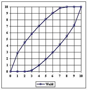
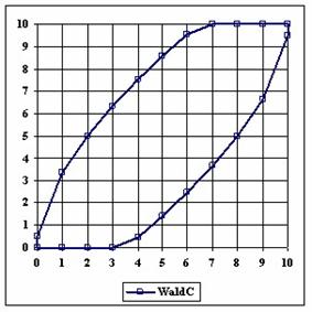
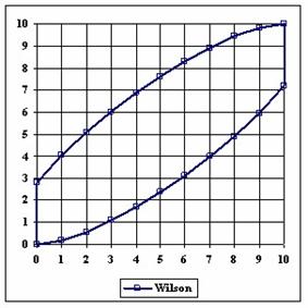
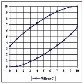
Figure 1. The lower and upper boundaries for proportion at X (0 ≤ X ≤ n) and n = 10
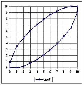
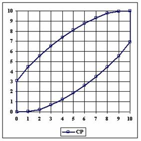
Figure 1. The lower and upper boundaries for proportion at X (0 ≤ X ≤ n) and n = 10
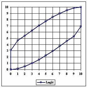
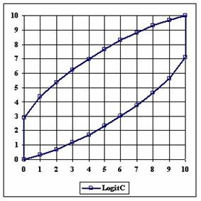
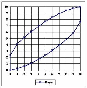
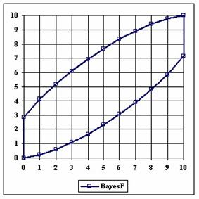
Figure 1. The lower and upper boundaries for proportion at X (0 ≤ X ≤ n) and n = 10
The contour plot using a method based on hypothesis of binomial distribution were graphically represented in figure 2 (graphical representation were created using a PHP program describe in the previous article of the series) [17]. With red color was represented the 0 values, with yellow the 0.5 values and with blue the 1 values. The intermediary color between the couplets colors (red, yellow, and blue) were represents using 18 hues.
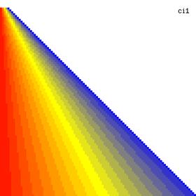
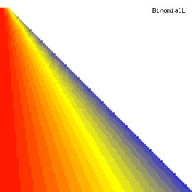
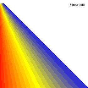
Figure 2. The contour plot for proportion (ci1) and its confidence intervals boundaries (BinomialL and BinomialU) computed with original Binomial method
The percentage of experimental errors depending on selected method and sample size are calculated and compared. The results are below. For a sample size equal with 10, the graphical representations of the experimental errors depending on selected method are in figure 3.
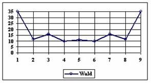
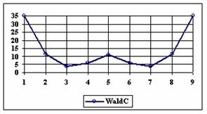
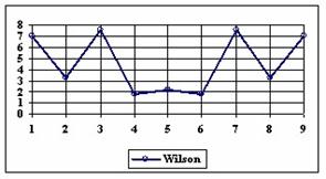
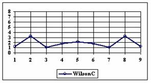
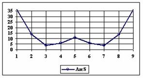
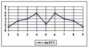
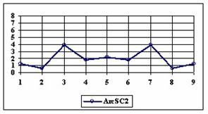
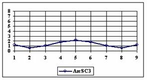
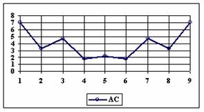
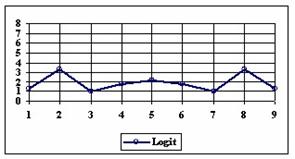
Figure 3. The percentages of the experimental errors for proportion for n=10 depending
on X (0 < X < n)
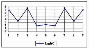
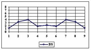
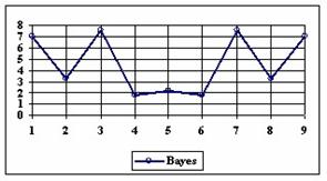


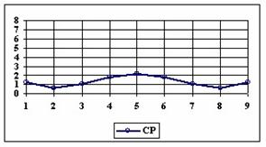
Figure 3. The percentages of the experimental errors for proportion for n=10 depending
on X (0 < X < n)
The graphics of the experimental errors percentages for a sample size of 30 using specified methods are in figure 4.
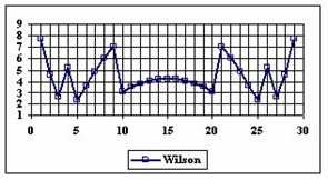
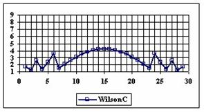
Figure 4. The percentage of the experimental errors for proportion for n = 30
depending on X (0 < X < n)
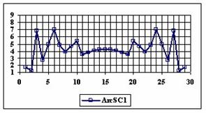
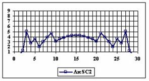
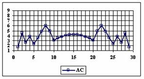
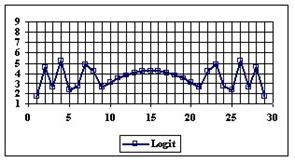
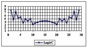
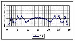
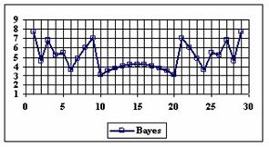
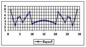
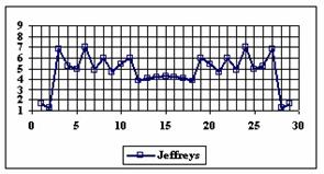
Figure 4. The percentage of the experimental errors for proportion for n = 30
depending on X (0 < X < n)
The graphical representations of the percentage of the experimental errors for a sample size equal with 100 using specified methods are in figure 5.
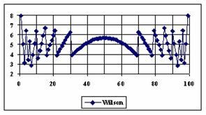

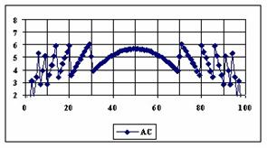
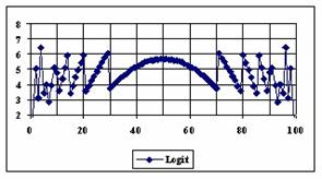
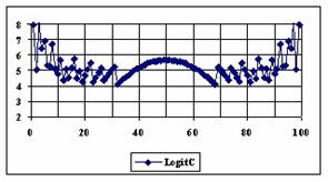
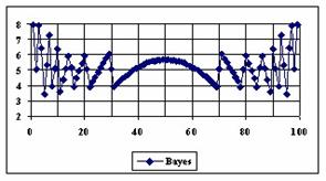
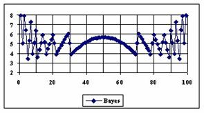
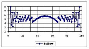
Figure 5. The percentages of the experimental errors for proportion for n = 100
depending on X (0 < X < n)
The diagrams of the experimental errors percentages for a sample size of 300 using specified methods are in figure 6.
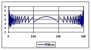
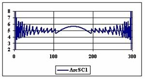
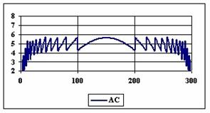
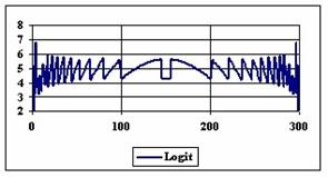
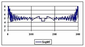
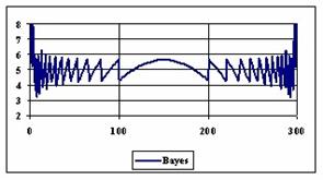
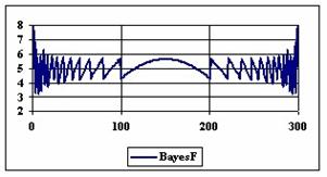
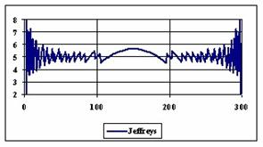
Figure 6. The percentages of the experimental errors for proportion for n = 300
depending on X (0 < X < n)
The methods Logit, LogitC and BayesF obtained the lowest standard deviation of the experimental errors (0.63%).
The graphical representations of the percentage of the experimental errors for a sample size equal with 1000 using specified methods are in figure 7.
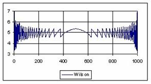
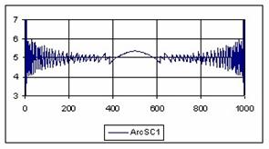
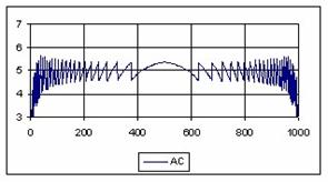
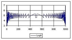
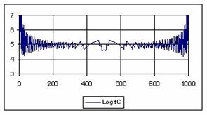
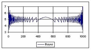
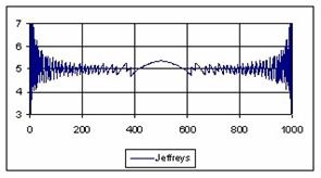
Figure 7. The percentage of the experimental errors fort n = 1000 depending on X (0<X<n)
For n = 1000 the Bayes method (0.39%) obtained the less standard deviations.
Figure 8 contain the subtraction and addition of the experimental standard deviation of the errors from the average of the experimental errors from n=4 to n=100.
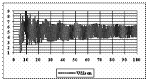
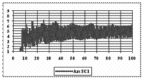
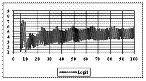
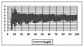
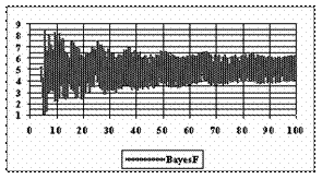
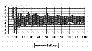
Figure 8. The [AM-STDEV, AM+STDEV] range for n = 4 to n = 100 depending on n, where AM is the average and STDEV is the standard deviation of experimental errors
The computed averages and the standard deviations of experimental errors for three ranges of sample sizes (4-10, 11-30, and 30-100), were presented in table 2.
|
n |
Wilson |
ArcSC1 |
Logit |
LogitC |
BayesF |
Jeffreys |
|
4-10 |
5.20 (2.26) |
2.36 (1.22) |
3.54 (2.02) |
4.90 (2.29) |
4.90 (2.29) |
5.69 (2.41) |
|
11-30 |
5.04 (1.93) |
4.17 (1.74) |
3.43 (1.19) |
4.88 (1.66) |
4.88 (1.88) |
4.78 (1.58) |
|
30-100 |
4.98 (1.20) |
4.76 (1.25) |
4.39 (1.03) |
5.07 (1.04) |
4.94 (1.18) |
4.92 (1.23) |
Table 2. The average of the experimental errors and standard deviation
for three ranges of n
The graphical representations of the subtraction and addition of the experimental standard deviation of the errors from the average of the experimental errors from n=101 to n=200 are in figure 9.
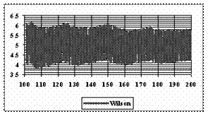
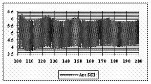
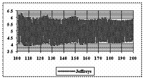
Figure 9. The [AM-STDEV, AM+STDEV] range for n = 100 to n = 200 depending on n, where AM is the average and STDEV is the standard deviation of experimental errors
The computed averages of the experimental errors and standard deviations of these errors, for some ranges of sample sizes are in table 3.
|
N |
Wilson |
ArcSC1 |
Logit |
LogitC |
BayesF |
Jeffreys |
|
101-110 |
4.96 (1.00) |
4.91(1.05) |
4.64 (0.90) |
5.10 (0.88) |
5.02 (0.99) |
5.04 (1.03) |
|
111-120 |
4.93 (0.92) |
4.87 (0.99) |
4.62 (0.82) |
5.09 (0.83) |
4.97 (0.89) |
4.95 (0.95) |
|
121-130 |
5.03 (0.93) |
5.01 (0.99) |
4.71 (0.87) |
5.10 (0.84) |
5.05 (0.88) |
5.02 (0.96) |
|
131-140 |
4.94 (0.88) |
4.86 (0.91) |
4.62 (0.80) |
5.03 (0.80) |
4.96 (0.84) |
4.91 (0.91) |
|
141-150 |
5.08 (0.85) |
4.99 (0.92) |
4.74 (0.83) |
5.14 (0.77) |
5.08 (0.84) |
5.06 (0.89) |
|
151-160 |
4.96 (0.86) |
4.88 (0.90) |
4.64 (0.80) |
5.01 (0.79) |
4.95 (0.84) |
4.96 (0.87) |
|
161-170 |
4.90 (0.79) |
4.95 (0.87) |
4.73 (0.76) |
5.09 (0.73) |
4.96 (0.77) |
4.97 (0.82) |
|
171-180 |
4.98 (0.81) |
5.00 (0.87) |
4.77 (0.76) |
5.10 (0.74) |
5.01 (0.77) |
5.04 (0.82) |
|
181-190 |
4.91 (0.78) |
4.89 (0.81) |
4.68 (0.70) |
5.03 (0.73) |
4.91 (0.75) |
4.94 (0.79) |
|
191-200 |
4.97 (0.75) |
4.94 (0.80) |
4.78 (0.70) |
5.14 (0.69) |
4.98 (0.71) |
5.01 (0.77) |
|
101-200 |
4.97 (0.86) |
4.93 (0.91) |
4.69 (0.79) |
5.08 (0.78) |
4.99 (0.83) |
4.99 (0.88) |
|
201-300 |
4.97 (0.69) |
4.96 (0.73) |
4.80 (0.65) |
5.07 (0.66) |
4.97 (0.67) |
5.01 (0.71) |
Table 3. Averages of the experimental error and standard deviation (parenthesis)
for proportion at n = 101 to n = 300
The contour plots of experimental error for each method when the sample size varies from 4 to 103 were illustrated in figure 10. On the contour plots were represented the error from 0% (red color) to 5% (yellow color) and ≥10% (blue color) using 18 hue. The vertical axis represent the values of sample size (n, from 4 to 103) and the horizontal axis the values of X (0 < X < n).

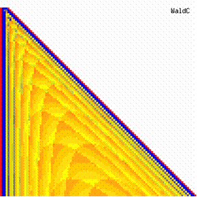

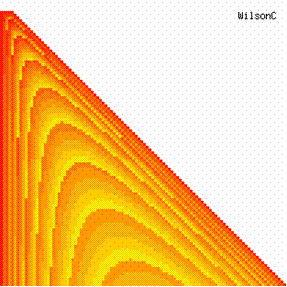
Figure 10. The contour plot of the experimental errors for 3 < n < 104
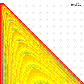
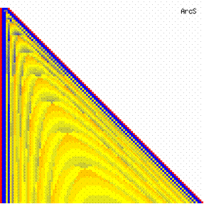
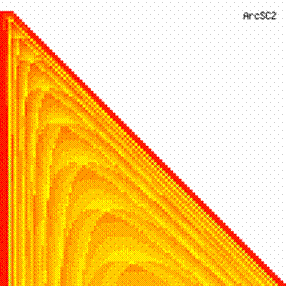
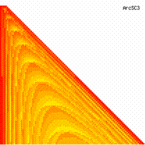
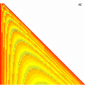
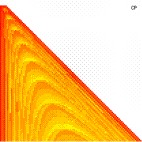
Figure 10. The contour plot of the experimental errors for 3 < n < 104
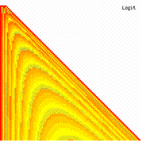
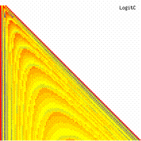
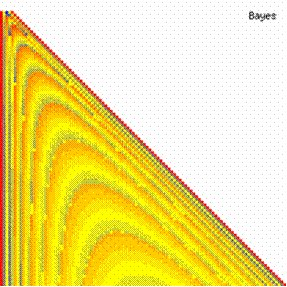
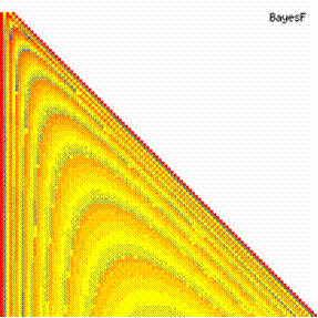
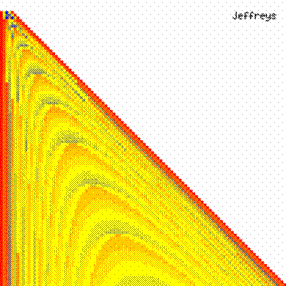
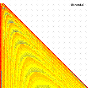
Figure 10. The contour plot of the errors for 3 < n < 104
A quantitative expression of the methods can be the deviations of the experimental errors for each proportion relative to the significance level α = 5% (Dev5) for a specified sample size (n), expression which was presented in material and methods section of the paper. The experimental results for n = 4..103, using Wilson, BayesF, Jeffreys, Logit, LogitC and Binomial methods, were taken and were assessed by count the best values of Dev5. The graphical representations of the frequencies are in figure 11.
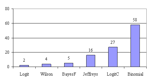
Figure 11. The best frequencies of deviations of the experimental error relative to the significant level (α = 5%) for n = 4...103
For the random experiment (random values for variable X from 1 to n-1, and random values for sample size n in the range 4 1000, the results are in tables 4-7 and graphical represented in figure 12.
In the figure 12 were represented with black dots the frequencies of the experimental error for each specified method; with green line the best frequencies of the errors interpolation curve with a Gauss curve (dIG(er)); with red line the Gauss curves of the average and standard deviation of the frequencies of the experimental errors (dMV(er)). The Gauss curve of the frequencies of experimental errors deviations relative to the significance level (d5V(er)) was represented with blue squares, and the Gauss curve of the standard binomial distribution of the imposed frequencies of the errors (pN(er, 10)) with black line.
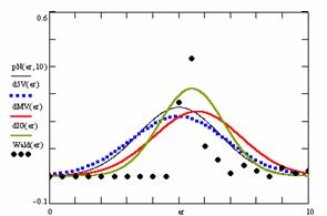
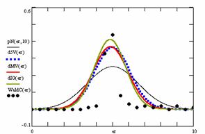
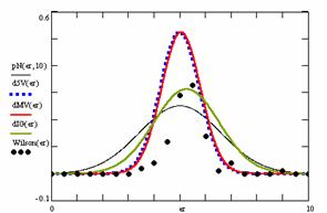
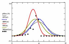
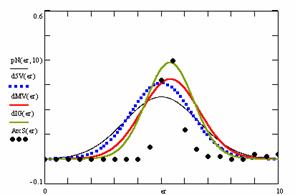
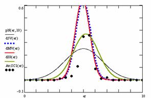

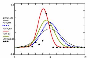
Figure 12. The pN(er, 10), d5V(er), dMV(er), dIG(er) and the frequencies
of the experimental errors for each specified method and random X, n
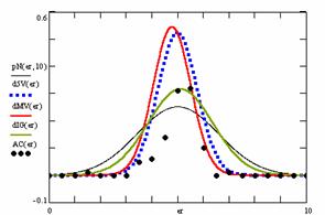
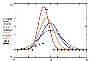

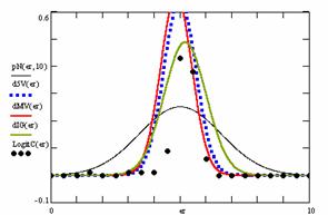
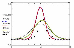
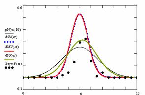
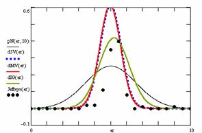
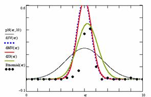
Figure 12. The pN(er, 10), d5V(er), dMV(er), dIG(er) and the frequencies
of the experimental errors for each specified method for random X, n
Table 4 contains the deviations of the experimental errors relative to significance level (Dev5), the absolute differences of the average of experimental errors relative to the imposed significance level (|5-M|), and standard deviations (StdDev). Table 5 contains the absolute differences of the averages that result from Gaussian interpolation curve to the imposed significance level (|5-MInt|), the deviations that result from Gaussian interpolation curve (DevInt), the correlation coefficient of interpolation (r2Int), and the Fisher point estimator (FInt).
|
Nr |
Method |
Dev5 |
Method |
|5-M| |
Method |
StdDev |
|
1 |
Binomial |
0.61 |
Binomial |
0.03 |
LogitC |
0.60 |
|
2 |
LogitC |
0.62 |
Jeffreys |
0.03 |
Binomial |
0.61 |
|
3 |
ArcSC1 |
0.62 |
Bayes |
0.03 |
ArcSC1 |
0.62 |
|
4 |
Jeffreys |
0.65 |
BayesF |
0.03 |
Jeffreys |
0.65 |
|
5 |
Bayes |
0.76 |
Wilson |
0.06 |
CP |
0.72 |
|
6 |
BayesF |
0.76 |
ArcSC1 |
0.08 |
AC |
0.73 |
|
7 |
Wilson |
0.76 |
WaldC |
0.12 |
Logit |
0.74 |
|
8 |
AC |
0.76 |
LogitC |
0.14 |
ArcSC2 |
0.74 |
|
9 |
Logit |
0.77 |
AC |
0.22 |
Bayes |
0.76 |
|
10 |
WaldC |
1.09 |
Logit |
0.23 |
BayesF |
0.76 |
|
11 |
CP |
1.16 |
ArcS |
0.40 |
Wilson |
0.76 |
|
12 |
ArcSC3 |
1.17 |
Wald |
0.72 |
ArcSC3 |
0.76 |
|
13 |
ArcSC2 |
1.18 |
ArcSC3 |
0.89 |
WilsonC |
0.84 |
|
14 |
ArcS |
1.30 |
CP |
0.90 |
WaldC |
1.08 |
|
15 |
WilsonC |
1.31 |
ArcSC2 |
0.91 |
ArcS |
1.23 |
|
16 |
Wald |
1.84 |
WilsonC |
1.01 |
Wald |
1.69 |
Table 4. Methods ordered by performance according to Dev5, |5-M| and StdDev criterions
|
Nr |
Method |
|5-MInt| |
Method |
DevInt |
Method |
r2Int |
FInt |
|
1 |
AC |
0.11 |
LogitC |
0.82 |
Wald |
0.62 |
31 |
|
2 |
Logit |
0.13 |
Binomial |
0.88 |
WilsonC |
0.65 |
36 |
|
3 |
WaldC |
0.14 |
Jeffreys |
0.95 |
ArcSC3 |
0.66 |
36 |
|
4 |
LogitC |
0.20 |
WaldC |
0.97 |
CP |
0.67 |
38 |
|
5 |
ArcSC1 |
0.22 |
CP |
0.97 |
ArcSC2 |
0.68 |
40 |
|
6 |
Jeffreys |
0.22 |
ArcS |
1.02 |
WaldC |
0.69 |
42 |
|
7 |
Bayes |
0.23 |
ArcSC3 |
1.08 |
Wilson |
0.71 |
47 |
|
8 |
BayesF |
0.23 |
ArcSC1 |
1.08 |
ArcS |
0.71 |
47 |
|
9 |
Wilson |
0.27 |
ArcSC2 |
1.11 |
AC |
0.71 |
47 |
|
10 |
Binomial |
0.27 |
Wald |
1.25 |
Logit |
0.71 |
47 |
|
11 |
ArcS |
0.38 |
AC |
1.26 |
Bayes |
0.71 |
47 |
|
12 |
ArcSC3 |
0.47 |
Logit |
1.27 |
BayesF |
0.71 |
47 |
|
13 |
ArcSC2 |
0.48 |
Wilson |
1.27 |
ArcSC1 |
0.72 |
50 |
|
14 |
CP |
0.49 |
Bayes |
1.29 |
Jeffreys |
0.74 |
54 |
|
15 |
Wald |
0.51 |
BayesF |
1.29 |
Binomial |
0.75 |
57 |
|
16 |
WilsonC |
0.60 |
WilsonC |
1.33 |
LogitC |
0.76 |
59 |
Table 5. The methods ordered by |5-Mint|, DevInt, r2Int and FInt criterions
The superposition between the standard binomial distribution curve and interpolation curve (pNIG), the standard binomial distribution curve and the experimental error distribution curve (pNMV), and the standard binomial distribution curve and the error distribution curve around significance level (pN5V) are in table 6.
|
Nr |
Method |
pNIG |
Method |
pNMV |
Method |
pN5V |
|
1 |
LogitC |
0.69 |
CP |
0.56 |
Binomial |
0.57 |
|
2 |
Binomial |
0.72 |
LogitC |
0.56 |
LogitC |
0.58 |
|
3 |
CP |
0.74 |
ArcSC2 |
0.57 |
ArcSC1 |
0.58 |
|
4 |
Jeffreys |
0.75 |
Binomial |
0.57 |
Jeffreys |
0.60 |
|
5 |
WaldC |
0.77 |
ArcSC1 |
0.57 |
Bayes |
0.66 |
|
6 |
ArcS |
0.77 |
ArcSC3 |
0.58 |
BayesF |
0.66 |
|
7 |
ArcSC3 |
0.78 |
WilsonC |
0.59 |
Wilson |
0.66 |
|
8 |
ArcSC2 |
0.79 |
Jeffreys |
0.60 |
AC |
0.66 |
|
9 |
ArcSC1 |
0.81 |
AC |
0.64 |
Logit |
0.67 |
|
10 |
WilsonC |
0.82 |
Logit |
0.64 |
WaldC |
0.82 |
|
11 |
Wald |
0.83 |
Bayes |
0.66 |
CP |
0.85 |
|
12 |
Wilson |
0.88 |
BayesF |
0.66 |
ArcSC2 |
0.86 |
|
13 |
Bayes |
0.88 |
Wilson |
0.66 |
ArcSC3 |
0.86 |
|
14 |
BayesF |
0.88 |
WaldC |
0.82 |
ArcS |
0.90 |
|
15 |
AC |
0.89 |
Wald |
0.82 |
WilsonC |
0.91 |
|
16 |
Logit |
0.89 |
ArcS |
0.84 |
Wald |
0.93 |
Table 6. Methods ordered by the pNING, pNMV, and pN5V criterions
|
Nr |
Method |
pIGMV |
Method |
pIG5V |
Method |
pMV5V |
|
1 |
WaldC |
0.95 |
WaldC |
0.93 |
Bayes |
0.99 |
|
2 |
ArcS |
0.91 |
ArcS |
0.84 |
BayesF |
0.99 |
|
3 |
Wald |
0.85 |
LogitC |
0.83 |
Binomial |
0.98 |
|
4 |
Binomial |
0.79 |
ArcSC2 |
0.83 |
Jeffreys |
0.98 |
|
5 |
Jeffreys |
0.79 |
ArcSC3 |
0.83 |
Wilson |
0.97 |
|
6 |
LogitC |
0.77 |
WilsonC |
0.82 |
WaldC |
0.96 |
|
7 |
CP |
0.77 |
CP |
0.81 |
ArcSC1 |
0.95 |
|
8 |
ArcSC3 |
0.77 |
Jeffreys |
0.80 |
LogitC |
0.91 |
|
9 |
ArcSC2 |
0.75 |
Wald |
0.78 |
AC |
0.88 |
|
10 |
Wilson |
0.75 |
Binomial |
0.78 |
Logit |
0.88 |
|
11 |
WilsonC |
0.75 |
Logit |
0.76 |
ArcS |
0.87 |
|
12 |
Bayes |
0.73 |
AC |
0.76 |
Wald |
0.83 |
|
13 |
BayesF |
0.73 |
Wilson |
0.74 |
ArcSC3 |
0.61 |
|
14 |
AC |
0.72 |
Bayes |
0.74 |
WilsonC |
0.60 |
|
15 |
Logit |
0.72 |
BayesF |
0.74 |
ArcSC2 |
0.60 |
|
16 |
ArcSC1 |
0.71 |
ArcSC1 |
0.73 |
CP |
0.59 |
Table 7. The confidence intervals methods ordered by the
pIGMV, pIG5V, and pMV5V criterions
The table 7 contains the percentages of superposition between interpolation Gauss curve and the Gauss curve of error around experimental mean (pIGMV), between the interpolation Gauss curve and the Gauss curve of error around imposed mean (α = 5%) (pIG5V) and between the Gauss curve experimental error around experimental mean, and the error Gauss curve around imposed mean α = 5% (pMV5V).
Discussions
The Wald method (figure 1) provides most significant differences in computing confidence intervals boundaries. If we exclude from discussion the Wald method and its continuity correction method (WaldCI method) we cannot say that there were significant differences between the methods presented; the graphical representation of confidence intervals boundaries were not useful in assessment of the methods.
As a remark, based on the figure 1, for n=10 there were five methods which systematically obtain the average of the experimental errors less then the imposed significant level (α = 5%): WilsonC (1.89%), ArcSC2 and ArcSC3 (1.93% for ArcSC2 and 1.31% for ArcSC2), Logit (1.89%), BS (2.52%) and CP (1.31%). For n = 10 the methods Wilson, LogitC, Bayes and BayesF obtained identical average of experimental errors (equal with 4.61%). We can not accept the experimental errors of Wald, WaldC, ArcS (the average of the experimental errors greater than imposed significant level α = 5%, respectively 17.33%, 13.69% and 15.53%); the ArcSC3 and the CP methods were obtained an average of the experimental errors equal with 1.31%. From the next experiments were excluded the specified above methods.
Looking at the graphical representations from figure 1 and 2, the upper confidence boundaries are the mirror image of the lower confidence boundaries.
For n = 30 the percentages of the experimental errors for the WilsonC (2.77%), ArcSC2 (3.27%) and BS (3.61%) methods were systematically less then the choused significant level (figure 4).
For n = 100 the Logit method obtain experimental errors greater than the imposed significant level of 5% (5.07% at X = 2, 6.43% at X = 4, and so on until X = 29), even if the error mean was less than 5% (4.71%). If we were looked at the average of the experimental errors and of standard deviations of them, the best mean were obtained by: Jeffreys (5.03%), ArcSC1 (4.96%), Wilson (5.07%) and BayesF (5.08%), and the best standard deviation by the methods: LogitC (0.83%), BayesF (0.91%), Logit (0.94%) and Bayes (0.95%).
Analyzing the percentage of the experimental errors for n=300, as we can saw from the graphical representation (figure 6) it result that the Wilson (5.03%), BayesF (5.04%) and ArcSC1 (5.06%) obtained the best average of the experimental errors.
For n = 1000 Wilson (5%), BayesF (5.01%) and ArcSC1(5.01%) obtained the best error mean (5.01%) and BayesF (0.37%) followed by Wilson, ArcSC1, Logit, LogitC.
Looking at the experimental results which present the average and the standard deviations of experimental errors for three specified ranges of sample sizes (see table 2) we remarked that Wilson had the most appropriate average of the experimental errors from the imposed significance level (α = 5%), and in the same time, the smallest standard deviation for n ≤ 10. For 10 < n ≤ 100 the best performance were obtained by the LogitC method.
For values of the samples size varying into the range 101 ≤ n < 201, cannot be observed any differences between Wilson, ArcSC1, Logit, LogitC, BayesF methods if we looked at the graphical representation (figure 9). Even if the graphical representation cannot observe the differences, these differences were real (see table 3). Analyzing the results from the table 3 we observed the constantly performance obtained by BayesF, with just two exceptions its average and standard deviations of the experimental errors were between the first three values. The LogitC method was the most conservative method if we looked at standard deviation, obtaining the first performance in 8 cases from 10 possible at n = 101 to n = 200. If we looked at the average of the errors, it were a little bit hard to decide which was the best, because ArcSC1, LogitC, BayesF and Jeffreys obtained at least two times the best performance reported to the choused significant level (α = 5%). Generally, if we looked at all interval (n = 101..300) it result that Jeffreys (4.991%) obtained the best error mean, followed by BayesF (4.989%).
Analyzing the deviation relative to the imposed significance level for each proportion for a specified sample size (n) (figure 11) some aspects are disclosure. The first observation was that the original method Binomial improved the BayesF and the Jeffreys methods even if, to the limit, the Binomial overlap on BayesF and Jeffreys (see the Binomial method formula):
![]() ,
, ![]()
The second observation was that the Binomial method obtained the best performance (with 58 apparitions, followed by LogitC with 27 apparitions).
The third observation which can be observed from the experimental data (cannot been seen from the graphical representation) was that for n > 30 Binomial was systematically the method with the best performance (had 54 apparition, followed by LogitC with 13; no apparition for other methods). Even more, starting with n = 67 and until n = 103 the Binomial method obtained every time the best deviations relative to the imposed significance level α = 5%. In order to confirm the hypothesis that for n ≥ 67 the Binomial method obtains the lowest deviations relative to the imposed significance level, the Dev5 for six sample sizes, from n = 104 to n = 109, were computed. For n=104 the Binomial method obtained the lowest deviations relative to the imposed significance level of the experimental errors (0.83, comparing with 0.90 obtained by the LogitC method, and BayesF method with 1.03, and Jefferys with 10.8). This characteristics was obtained systematically (0.76 for n=105, 0.77 for n=106, 0.76 for n=107, 0.75 for n=108, 0.75 for n=109). The observation described above confirm the hypothesis that Binomial method obtained the smallest deviations relative to the significance level α = 5%.
The best three methods reported in specialty literature that obtain the greatest performance in our experiments are in table 8.
|
n |
Method |
|
4-10 |
Wilson, LogitC, BayesF |
|
11-30 |
LogitC, BayesF, Wilson |
|
31-100 |
LogitC, BayesF, Wilson |
|
101-300 |
BayesF, LogitC, Wilson |
Table 8. The best three methods depending on n
Looking at the results obtained from the random samples (X, n random numbers, n range 4..1000 and X range 1..n-1), it can be remarked that the Binomial method obtain the closed experimental error mean to the imposed mean (α = 5%). The LogitC method obtains the lowest standard deviations of the experimental errors (table 4).
The Agresti-Coull was the method which obtained the closed interpolation mean to the imposed mean (table 5), followed by the Logit method; LogitC (closely followed by the Binomial method) was the method with the lowest interpolation standard deviation. The LogitC method followed by the Binomial method provides the best correlation between theoretical curve and experimental data.
It can observed analyzing the results presented in the table 6, that the Logit and the Agresti-Coull methods, followed by the Bayes, BayesF and Wilson were the methods that presented the maximum superposition between the curve of interpolation and the curve of standard binomial distribution. With ArcS method obtains the maximum superposition between the curve of standard binomial distribution and the curve of experimental errors.
The maximum superposition between the Gauss curve of interpolation and the Gauss curve of errors around experimental mean is obtain by the WaldC method, followed by the ArcS, the Wald and the Binomial methods (table 7). The WaldC method obtained the maximum superposition between the Gauss curve of interpolation and the Gauss curve of errors around imposed mean.
The Bayes and the BayesF methods obtained the maximum superposition between experimental error Gauss curve distribution and the error Gauss curve distribution around imposed mean.
Conclusions
Choosing a specified method of computing the confidence intervals for a binomial proportion depend on an explicit decision whether to obtain an average of the experimental errors closed to the imposed significance level or to obtain the lowest standard deviation of the errors for a specific sample size.
In assess of the confidence intervals for a binomial proportion, the Logit and the Jeffreys methods obtain the lowest deviations of experimental errors relative to the imposed significance level and the average of the experimental errors smaller than the imposed significance level. Thus, if we look after a confidence intervals which to assure the lowest standard deviation of the errors we will choose one of these two methods.
If we want a method which to assure an average of the experimental error close to the imposed significance level, then the BayesF method could be choose for a sample size on the range 4 ≤ n ≤ 300.
The Binomial method obtains the best performance in confidence intervals estimation for proportions using random sample size from 4 to 1000 and random binomial variable from 1 to n-1 and systematically obtains the best overall performance starting with a sample size greater than 66.
Acknowledgements
First author is thankful for useful suggestions and all software implementation to Ph. D. Sci., M. Sc. Eng. Lorentz JÄNTSCHI from Technical University of Cluj-Napoca.
References