Leonardo Electronic Journal of Practices and Technologies
Issue 03, p. 001-030
Installing and Testing a Server Operating System
Lorentz JÄNTSCHI
Technical University of Cluj-Napoca, Romania,
http://lori.academicdirect.ro
Abstract
The paper is based on the experience of the author with the FreeBSD server operating system administration on three servers in use under academicdirect.ro domain. The paper describes a set of installation, preparation, and administration aspects of a FreeBSD server. First issue of the paper is the installation procedure of FreeBSD operating system on i386 computer architecture. Discussed problems are boot disks preparation and using, hard disk partitioning and operating system installation using a existent network topology and a internet connection. Second issue is the optimization procedure of operating system, server services installation, and configuration. Discussed problems are kernel and services configuration, system and services optimization. The third issue is about client-server applications. Using operating system utilities calls we present an original application, which allows displaying the system information in a friendly web interface. An original program designed for molecular structure analysis was adapted for systems performance comparisons and it serves for a discussion of Pentium, Pentium II and Pentium III processors computation speed. The last issue of the paper discusses the installation and configuration aspects of dial-in service on a UNIX-based operating system. The discussion includes serial ports, ppp and pppd services configuration, ppp and tun devices using.
Keywords
Server operating systems, Operating system configuration, Server services, Client-server applications, Dial-in server, System testing
Introduction
UNIX is an interactive time-sharing operating system invented in 1969 by Ken Thompson after Bell Labs left the Multics project, originally so he could play games on his scavenged PDP-7. The time-sharing is an operating system feature allowing several users to run several tasks concurrently on one processor, or in parallel on many processors, usually providing each user with his own terminal for input and output; time-sharing is multitasking for multiple users. Dennis Ritchie, the inventor of {C}, is considered a co-author of the UNIX system. The turning point in UNIX's history came when it was reimplemented almost entirely in C during 1972 - 1974, making it the first source-portable OS. UNIX subsequently underwent mutations and expansions at the hands of many different people, resulting in a uniquely flexible and developer-friendly environment. By 1991, UNIX had become the most widely used multi-user general-purpose operating system in the world. Many people consider this the most important victory yet of hackerdom over industry opposition. Another point of view expresses a UNIX conspiracy. According to a conspiracy theory long popular among ITS and TOPS-20 fans, UNIX's growth is the result of a plot, hatched during the 1970s at Bell Labs, whose intent was to hobble AT&T's competitors by making them dependent upon a system whose future evolution was to be under AT&T's control. This would be accomplished by disseminating an operating system that is apparently inexpensive and easily portable, but also relatively unreliable and insecure (to require continuing upgrades from AT&T). In this view, UNIX was designed to be one of the first computer viruses (see virus) - but a virus spread to computers indirectly by people and market forces, rather than directly through disks and networks. Adherents of this UNIX virus theory like to cite the fact that the well-known quotation UNIX is snake oil was uttered by DEC president Kenneth Olsen shortly before DEC began actively promoting its own family of UNIX workstations. UNIX is now offered by many manufacturers and is the subject of an international standardization effort. Unix-like operating systems include Debian, Linux and LinwowsOS, AIX, GNU, HP-UX, OSF and Solaris, BSD/OS, NetBSD, OpenBSD and FreeBSD (with TrustedBSD and PicoBSD project variations)[1]. FreeBSD (FreeBSD is a registered trademark of Wind River Systems, Inc. and this is expected to change soon) is an advanced operating system for x86 compatible, AMD64, Alpha, IA-64, PC-98 and UltraSPARC architectures. It is derived from BSD/OS (BSD is a registered trademark of Berkeley Software Design, Inc.), the version of UNIX (UNIX is a registered trademark of The Open Group) developed at the University of California, Berkeley. The FreeBSD operating system is developed and maintained by a large team of individuals. While you might expect an operating system with these features to sell for a high price, FreeBSD is available free of charge and comes with full source code. NetBSD's focus lies in providing a stable, multiplatform, and research oriented operating system. NetBSD's portability leads it to run on 33 platforms as of January 2001. Even more impressive is the list of hardware including traditional modern server equipment like standard Intel-based PCs, Compaq's Alpha, or Sun Microsystem's SPARC architectures. Older server and workstation class hardware like the Digital Equipment Corporation's VAX hardware, Apple's Macintosh computers based on Motorola's 68000 processor series are also support. But what really sets NetBSD apart is its support for more exotic hardware including Sega's Dreamcast, Cobalt Network's server appliances, and George Scolaro's and Dave Rand's PC532 hobbyist computer. NetBSD's dedication to portability has led the way for other operating systems. When the FreeBSD group began porting to the Alpha platform, the initial work from the NetBSD project provided the foundation. With new FreeBSD ports to both the PowerPC and SPARC platforms under way, work from NetBSD is being used again. Linux has benefited from NetBSD's experience as well. The special booter used by NetBSD on the 68000-series Macintosh computers was modified and became the Penguin booter used to launch Linux on these systems. Finally, NetBSD's largest contribution to other systems lies in acting as a springboard for the OpenBSD operating system. OpenBSD diverged from NetBSD around the release of NetBSD 1.1 in November of 1995. OpenBSD's first release came a year later when OpenBSD 2.0 was released in October of 1996. OpenBSD quickly began focusing on producing the most secure operating system available. Taking advantage of his Canadian residency, de Raadt realized United States munitions export laws did not hamper him, allowing inclusion of strong cryptography including RSA, Blowfish, and other advanced algorithms. A modified version of the Blowfish algorithm is now in use for encrypting user passwords by default. OpenBSD developers also spear-headed the development of OpenSSH, a multiplatform clone of the wildly popular protocol for secures communications. OpenBSD also advanced the state of code auditing. Beginning in 1996, the OpenBSD team began a line-by-line analysis of the entire operating system searching for security holes and potential bugs. UNIX systems have been plagued for decades by the use of fixed-sized buffers. Besides being inconvenient for the programmer, they have lead to numerous security holes like the fingerd exploit in 4.2BSD. Other security holes relating to mishandling temporary files are easily caught. OpenBSD's groundbreaking audit has also discovered security-related bugs in related operating systems including FreeBSD, NetBSD, and mainstream System V derivatives. However, the nature of this process allows general coding mistakes not relating to security to be caught and corrected, as well. Additionally, a number of bugs in Ports, or third party applications have been discovered through this process. Referring to FreeBSD, perhaps what sets FreeBSD apart most is its technical simplicity. The FreeBSD installation program is widely regarded as the simplest UNIX installation tool in existence. Further, its third party software system, the Ports Collection, has been modeled by NetBSD and OpenBSD and remains the most powerful application installation tool available. Through simple one-line commands, entire applications are downloaded, integrity checked, built, and installed making system administration amazingly simple. The most important feature of a server system is system services. Most of the services in a server system are provided through a program or process that sits idly in the background until it is invoked to perform its task, called daemons[2]. The daemon word come from the mythological meaning, later rationalized as the acronym Disk And Execution MONitor[3]. A daemon is program that is not invoked explicitly, but lays dormant waiting for some condition(s) to occur. The idea is that the perpetrator of the condition need not be aware that a daemon is lurking (though often a program will commit an action only because it knows that it will implicitly invoke a daemon). For example, under ITS writing a file on the LPT spooler's directory would invoke the spooling daemon, which would then print the file. The advantage is that programs wanting files printed need neither compete for access to, nor understand any idiosyncrasies of, the LPT. They simply enter their implicit requests and let the daemon decide what to do with them. Daemons are usually spawned automatically by the system, and may either live forever or be regenerated at intervals. UNIX systems run many daemons, chiefly to handle requests for services from other hosts on a network. Most of these are now started as required by a single real daemon, inetd, rather than running continuously. Examples are cron (local timed command execution), rshd (remote command execution), rlogind and telnetd (remote login), ftpd, nfsd (file transfer), lpd (printing)[4]. The discussed services are Internet domain name server (named,[5]?query=named]), Internet super-server (inetd, [5?query=inetd]), OpenSSH SSH daemon (sshd, [5?query=sshd]), Internet file transfer protocol server (ftpd, [5?query=ftpd]), Apache hypertext transfer protocol server (httpd, [5?query=httpd]), proxy caching server (squid, [5?query=squid), the MySQL server demon (mysqld, [5?query=mysqld]) and PHP sub-service (post processed hypertext[6]). Many system information applications are available. Looking at FreeBSD ports, a good application is phpSysInfo[7]. The problem that appears is that, not always, the system information application makes the updates and a set of problems can appear, especially for CURRENT systems[8]. In order to create a web application for system information, at least our system must have a web server installed. If we propose to test the performances of computer architecture, first we must look at the hardware specifications. Because the application requires using of the system functions, a good idea is to use software with Perl support. Many reasons lead to the PHP language for the applications implementation[9]. Two methods of dialing into a machine to get access to the Internet are widely used. If you dial in and log on as usual (on UNIX you see "login:" and shell prompt or on MPE you type "HELLO" and get a colon prompt), your computer is not directly connected to the Internet, so it cannot send network packets from your PC to the Internet. In this case, you will have to use Lynx to access the WWW. If you dial-in using SLIP (Serial Line IP) or PPP (Point-to-Point Protocol), your computer becomes part of the Internet, which means it can send network packets to and from the Internet. In this case, you can use graphical browsers like Mosaic or Netscape to access the WWW. The Internet Adapter is supposed to allow users with only shell account access to obtain a SLIP connection[10]. To install and configure a digital modem[11] is quite different from analog modems[12]. Until the digital phone lines take the place of analog ones, the analog modems will stay on base of the most dial-up connections. The present paper is focused on analog modems software configuration to work as a dial-in server. A FreeBSD 5.2-CURRENT operating system is the support for the dial-in server service. From the start, an appreciation is necessary: the current modems standards are V.30, V.34, V.90 and V.92. Considering the most advanced standard, through an analog phone line we can get at most 4.8 Kb/s as rate of compressed data upload transfer. The dial-in server installation requires, in most of the cases, system configurations and in some cases, kernel recompilations, to support the modem. To know which modem is supported on the system, a good idea is to consult the Release Notes of the system. To avoid any compatibility problems, a good idea is to chouse an external modem.
Operating System Installing Procedure
First step in FreeBSD operating system installation is to create a boot disk set, depending on machine type. If we are using a Personal Computer, based on i386 computer architecture, a disk boot set can be found at:
ftp://ftp.freebsd.org/pub/FreeBSD/releases/i386/5.2-RELEASE/floppies/
For 1.44Mb floppies, all that we have to do is to download at least kern.flp and mfsroot.flp files. If the planned computer to be a server has exotic or old components, is possible to need also the drivers.flp file. If we use a DOS/Windows operating system type, to create the boot disks is necessary to download and use an image file installation program, which can be found at the address:
ftp://ftp.freebsd.org/pub/FreeBSD/tools/
We can use any of fdimage.exe or rawrite.exe to create the disks. For fdimage.exe the commands (DOS commands) are (assuming that we use a: drive):
fdimage f 1.44M kern.flp a:
(and similarly for mfsroot.flp and drivers.flp files).
If we use a UNIX operating system type, we can use dd program for disks creation:
dd if=kern.flp of=/dev/floppy
(and similarly for mfsroot.flp and drivers.flp files)
After the boot disks creation, we must boot from kern.flp floppy and mfsroot.flp floppy the FreeBSD operating system. Kernel and SysInstall utility are automatically loaded and after that, we have two consoles (alt+F1 and alt+F2 respectively). The second console is for DEBUG messages. In the DEBUG console we can watch how modules are loaded. In this moment, a good idea is to look at the DEBUG console to assure that our network card is proper identified and used. In our installation procedure, we use a 3COM network card (3c905B) and the DEBUG messages are:
DEBUG: loading module if_xl.ko
xl0: <3Com 3c905B-TX Fast Etherlink XL>
	port 0x1000-0x107f mem 0x40400000-0x4040007f irq 17 at device 9.0 on pci2
xl0: Ethernet address: 00:04:76:9d:2e:02
miibus0: <MII bus> on xl0
xlphy0: <3Com internal media interface> on miibus0
xlphy0: 10baseT, 10baseT-FDX, 100baseTX, 100baseTX-FDX, auto
Until this step, only CD file system, SYSV messages queue, shared memory and semaphores, serial and network modules are loaded. If is necessary, at this point we have the option to load a specific module from drivers.flp floppy. At this point, SysInstall utility load FDISK partion editor and we must create a FreeBSD partition using a set of commands:
A Use entirely disk
C Create slice
S set bootable
Q finish
F Dangerously dedicated mode (purposely undocumented)
If we chouse to use entirely disk, the choice is simple (A, S, Q). After FDISK partion editor, we can chouse to select a boot manager utility (from three possibilities):
Install FreeBSD Boot Manager FreeBSD system will select the booted operating system;
Install Standard Boot Manager (MBR) disable other operating system boot managers;
Leave Master Boot untouched if we want that other existing boot manager to manage booting.
An observation is useful: for PC-DOS users the last option allow to exist both operating systems on same machine. After Boot Manager on disk selection, FreeBSD Disklabel editor are invoked and we must specify at least two partitions, one for root mount point (/) and one for swap (swap). A good idea is to specify the swap size at least 2*memory. The SysInstall utility let us now to select the installation options such as preinstalled binaries, services and documentation. If we plan to update and/or upgrade our system after the installation, a good idea is to select a minimal configuration. The installation of operating system continues with installation media selection. If our computer is connected to the Internet via a high-speed communication line, a good idea is to install the system directly from internet. Anyway, now we have the options to install from a CD, from a DOS partition, over Network File Server, existing file system, floppy disk set, SCSI or QIC tape, and from a FTP server. If we chouse the installation from a FTP server, we must know the network topology to do this. Three possibilities are there:
FTP (install from an FTP server),
FTP Passive (Install from an FTP server through a firewall)
HTTP (Install from an FTP server through an http proxy).
Anyway, the host configuration is necessary and the configuration will be made for used communication device (in our case xl0). A selection from three protocols it must be done (IPv6, IPv4 or DHCP) depending on network topology. In our case, IPv4 is the proper choice. The host (vl), the domain (academicdirect.ro), the IPv4 gateway (193.226.7.211), name server (193.226.7.211), IPv4 address (193.226.7.200) and net mask (255.255.255.0) must be specified. If we chouse to install via a proxy server, we also must specify the proxy address (193.226.7.211) and port (3128). After the communication interface configuration, the SysInstall utility load all required modules (see DEBUG console) and make the internet connection for installation. At the end of system installation, we have the option to preinstall a set of packages in our system. Anyway, the option can be ignored, since the SysInstall utility is also preinstalled in our system and can be invoked anytime after reboot. Some final configurations can be specified at the end of the installation (such as boot services, root password, group and user management). Only root password is obligatory (root are the superuser in FreeBSD system). After reboot, we have a FreeBSD system on our machine.
Operating System Configuration
After the system installation, we can configure it. Many configurations can be done. We can start to download now all system sources. A utility called cvsup can be used for this task. CVSup is a software package for distributing and updating source trees from a master CVS repository on a remote server host. The FreeBSD sources are maintained in a CVS repository on a central development machine in California. With CVSup, FreeBSD users can easily keep their own source trees up to date. Using SysInstall utility, we can fetch the cvsup program in the same way as we installed the system, from internet via FTP protocol (sysinstall/Configure/Packages/ ... logging... /devel/cvsup-without-gui-16.1h). After the cvsup installation, a configuration file (let us call it configuration_file) must be created (or edited from /usr/share/examples/cvsup/) and must contain the host (this specifies the server host which will supply the file updates), the base (this specifies the root where CVSup will store information about the collections you have transferred to our system), the prefix (this specifies where to place the requested files), and the desired release (version). Other options are also benefit:
*default host=cvsup.FreeBSD.org
*default base=/usr
*default prefix=/usr
*default release=cvs
*default delete use-rel-suffix
*default compress
src-all tag=.
ports-all tag=.
doc-all tag=.
cvsroot-all tag=.
Sources can be fetched separately (such as src-base) or entirely (such as src-all). Tag option is used to fetch one specific version of the sources (when . means CURRENT versions). In addition, the date option can be used (as example: src-all tag=RELENG_4 date=2000.08.27.10.00.00). Fetching procedure can be done now from a text console, using a simple command:
cvsup -g -L 2 configuration_file
or from a graphical console (X-based) using the command:
cvsup configuration_file
Recompilation and System Optimization
The kernel is the core of the FreeBSD operating system. It is responsible for managing memory, enforcing security controls, networking, disk access, and much more. While more and more of FreeBSD become dynamically configurable, it is still occasionally necessary to reconfigure and recompile the kernel. Building a custom kernel is one of the most important rites of passage nearly every UNIX user must endure. This process, while time consuming, will provide many benefits to your FreeBSD system. Unlike the GENERIC kernel, preinstalled in our system, which must support a wide range of hardware, a custom kernel only contains support for your PC's hardware. This has a number of benefits, such as:
faster boot time (since the kernel will only probe the hardware you have on our system, the time it takes your system to boot will decrease dramatically);
less memory usage (a custom kernel often uses less memory than the GENERIC kernel, which is important because the kernel must always be present in real memory; for this reason, a custom kernel is especially useful on a system with a small amount of RAM);
additional hardware support; a custom kernel allows you to add in support for devices such as sound cards, which are not present in the GENERIC kernel.
If we follow the acquiring procedure of the sources exactly, we can found for the kernel configuration a set of predefined configuration files at the location:
/usr/src/sys/i386/conf/
If the sources version fit with our system then the GENERIC file using must produce same kernel and modules with the existent ones. The idea is to optimize the kernel at compilation time. The kernel can be configured in a configuration file using the prescriptions that can be found in following files:
GENERIC, Makefile, NOTES (/usr/src/sys/i386/conf/),
NOTES from /usr/src/sys/conf/
README and UPDATING from /usr/src/.
Additionally, we can create the LINT file which contain additional kernel configuration options from NOTES files with make utility (cd /usr/src/sys/i386/conf/ && make LINT). In the optimizing process of the kernel, a good idea is to look at the system characteristics detected by the GENERIC kernel using the dmesg utility. After the reading of these files and understanding of the nature of the process, first step is to create our own kernel configuration file (cd /usr/src/sys/i386/conf/ && cp GENERIC VL). We can now edit this file (using as example ee utility) and set the CPU type (see dmesg | grep CPU), ident (same with file name, VL), debug and SYSV options (enable or disable), console behavior (as example:
options SC_DISABLE_REBOOT;
options SC_HISTORY_SIZE=2000;
options SC_MOUSE_CHAR=0x3;
options MAXCONS=5;
options SC_TWOBUTTON_MOUSE
). Most of the essential options are well documented and we cannot miss. Anyway, a large set of network devices can be excluded from the kernel. To find which device driver is using in the system for network adapter management we can look again at the boot messages (dmesg | grep Ethernet). Supposing that we have finished our kernel configuration, the next step is to configure-it according with the new configuration file:
cd /usr/src/sys/i386/conf/ && config VL
The next three steps can be emerged in one composed command:
cd ../compile/VL && make depend && make && make install
The && operator has advantage that if we miss something and a error is detected, the following commands are aborted. Anyway, supposing that we configured, compiled and installed the kernel, but the system do not boot. This is not necessary a problem. BootLoader utility allows us to repair this damage. At the boot, hit any key except for the Enter key; the system lead us in a shell; following commands solve the problem:
unload kernel
load /boot/kernel.old/kernel
boot
If we want to restore the old configuration:
rm fr /boot/kernel
cp fr /boot/kernel.old/kernel /boot/kernel
To prevent that also kernel.old to be loosed in recompilation process, a good idea is to save the GENERIC kernel:
cp fr /boot/kernel /boot/kernel.GENERIC
The optimization process of kernel in generally reduces the kernel size (ls al):
-r-xr-xr-x 1 root wheel 5934584 Feb 8 02:55 /boot/kernel.GENERIC/kernel
-r-xr-xr-x 1 root wheel 3349856 Feb 14 00:10 /boot/kernel/kernel
The System Services
The kernel configuration process allowed us to define console behavior (to disable cltr+alt+del reboot sequence), to increase the amount of free memory available for processes and increase the system speed. Now can begin to install and configure the server services. The named service. Name servers usually come in two forms: an authoritative name server, and a caching name server. An authoritative name server is needed when:
one wants to serve DNS information to the world, replying authoritatively to queries;
a domain, such as academicdirect.ro, is registered (to RNC,[13]) and IP addresses need to be assigned to hostnames under it;
an IP address block requires reverse DNS entries (IP to hostname).
a backup name server, called a slave, must reply to queries when the primary is down or inaccessible.
A caching name server is needed when:
a local DNS server may cache and respond more quickly than querying an outside name server;
a reduction in overall network traffic is desired (DNS traffic has been measured to account for 5% or more of total Internet traffic).
A named configuration file resides in /etc/namedb/ directory, and to start automatically at boot, the /etc/rc.conf file must contain:
named_enable="YES"
For a real name server, at least following lines (from /etc/namedb/named.conf file) must fit with our system (academicdirect.ro):
zone "academicdirect.ro"
	{
		type master;
		file "academicdirect.ro";
	};
So, in academicdirect.ro file we must specify the zone. At least following lines must fit (see also [13]):
$TTL 3600
academicdirect.ro. IN SOA ns.academicdirect.ro. root.academicdirect.ro. (
	2004020902; Serial
	3600; Refresh
	1800; Retry
	604800; Expire
	86400; Minimum TTL
	)
@ IN NS ns.academicdirect.ro. ; DNS Server
@ IN NS hercule.utcluj.ro. ; DNS Server
localhost IN A 127.0.0.1; Machine Name
ns IN A 193.226.7.211; Machine Name
mail IN A 193.226.7.211; Machine Name
@ IN A 193.226.7.211; Machine Name
To properly create the local reverse DNS zone file, following command are necessary:
cd /etc/namedb && sh make-localhost
The inetd service manages (start, restart, and stop) a set of services (according with Internet server configuration database /etc/inetd.conf), for both IPv4 and IPv6 protocols, such as:
ftp stream tcp4 nowait root /usr/libexec/ftpd ftpd l # ftp IPv4 service
ftp stream tcp6 nowait root /usr/libexec/ftpd ftpd l # ftp IPv6 service
ssh stream tcp4 nowait root /usr/sbin/sshd sshd -i -4 # ssh IPv4 service
ssh stream tcp6 nowait root /usr/sbin/sshd sshd -i -6 # ssh IPv6 service
finger stream tcp4 nowait/3/10 nobody /usr/libexec/fingerd fingerd s # finger IPv4
finger stream tcp6 nowait/3/10 nobody /usr/libexec/fingerd fingerd s # finger IPv6
ntalk dgram udp wait tty:tty /usr/libexec/ntalkd ntalkd # talk
pop3 stream tcp4 nowait root /usr/local/libexec/popper popper # pop3 IPv4 service
pop3 stream tcp6 nowait root /usr/local/libexec/popper popper # pop3 IPv6 service
In some cases, is possible that ined service do not start. A solution is manual starting of a specific service (/usr/libexec/ftpd -46Dh) or creating of an executable shell script and place-it in an rc.d directory:
-r-xr-xr-x 1 root wheel 60 Feb 12 12:34 /usr/local/etc/rc.d/ftpd.sh (ls al)
/usr/libexec/ftpd -46Dh && echo -n ' ftpd' (ftpd.sh file content)
In other cases, may be we want to use another daemon for a specific service (such as /etc/rc.d/sshd shell script for sshd service). The Hypertext Transfer Protocol Server can be provided also by many applications such as httpd (apache@apache.org), bozohttpd (Janos.Mohacsi@bsd.hu), dhttpd (gslin@ccca.nctu.edu.tw), fhttpd (ports@FreeBSD.org), micro_httpd (user@unknown.nu), mini_httpd (se@FreeBSD.org), tclhttpd (mi@aldan.algebra.com), thttpd (anders@FreeBSD.org), w3c-httpd (ports@FreeBSD.org), but full featured and multiplatform capable remains httpd from Apache[14]. The most important feature of Apache web server is PHP language modules support, which transform our web server into a real client-server interactive application. The FreeBSD operating system offers a strong database support with MySQL database server (very fast, multi-threaded, multi-user and robust SQL,[15], mysqld daemon). Some configurations are very important for services behavior. Let us to exemplify some of the services configuration options. For httpd service (/usr/local/etc/apache2/httpd.conf):
Listen 80 # httpd port
<IfModule mod_php5.c>
	AddType application/x-httpd-php .php
	AddType application/x-httpd-php-source .phps
</IfModule> # not included by the default but required to work
ServerName vl.academicdirect.ro:80
For PHP module (/usr/local/etc/php.ini):
precision = 14 ; Number of significant digits displayed in floating point numbers
expose_php = On ; PHP may expose the fact that it is installed on the server
max_execution_time = 3000 ; Maximum execution time of each script, in seconds
max_input_time = 600 ; Maximum amount of time for parsing request data
memory_limit = 128M ; Maximum amount of memory a script may consume
post_max_size = 8M ; Maximum size of POST data that PHP will accept
file_uploads = On ; Whether to allow HTTP file uploads
upload_max_filesize = 8M ; Maximum allowed size for uploaded files
display_errors = On ; For production web sites, turn this feature Off
For squid service (/usr/local/etc/squid/squid.conf):
http_port 3128 # The socket addresses where Squid will listen for client requests
auth_param basic children 5
auth_param basic realm Squid proxy-caching web server
auth_param basic credentialsttl 2 hours
read_timeout 60 minutes # The read_timeout is applied on server-side connections
acl all src 0.0.0.0/0.0.0.0
acl localhost src 127.0.0.1/255.255.255.255
acl to_localhost dst 127.0.0.0/8
acl SSL_ports port 443 563
acl Safe_ports port 80 # http
acl Safe_ports port 21 # ftp
acl Safe_ports port 1025-65535 # unregistered ports
acl Safe_ports port 591 # filemaker
acl Safe_ports port 777 # multiling http
acl CONNECT method CONNECT
acl network src 172.27.211.1 172.27.211.2 193.226.7.200 192.168.211.2
http_access allow network acl ppp src 192.168.211.0/24
http_access allow ppp
http_access deny all
PHP Language Capabilities
The PHP language has a rich strong functions library, which can significantly shorten the algorithm design and implementation. In the following, some of them (already tested ones) are presented, using sequences of our first program for system information:
$b = preg_split("/[\n]/",$a,-1,PREG_SPLIT_NO_EMPTY);//require pcre module
// split string into an array using a perl-style regular expression as a delimiter
$c = explode(" ",$b[$i]);
// splits a string on string separator and return array of components
$c = str_replace("<","(",$c);
//replaces all occurrences of first from last with second
$a=`uptime`; //PHP supports one execution operator: backticks (``)
A set of shell execution applications are used with execution operator:
$a=`cat /etc/fstab | grep swap`; // swap information
$a=`uptime`; // show how long system has been running
$a =`top -d2 -u -t -I -b`; // display information about the top CPU processes
$a =`dmesg`; // display the system message buffer
$a=`netstat -m`; // show network status
$aa =`df -ghi`; // display free disk space
$s=`netstat -i`; // show network status
$s=`pkg_info`; // a utility for displaying information on software packages
The second application (hin.php file) is of client-server architecture and uses a class structure to define a chemical molecule:
define("l_max_cycle",16);
class m_c{
	var $a;//number of atoms var
	$b;//number of bonds var
	$c;//molecule structure var
	$e;//seed var
	$f;//forcefield var
	$m;//molecule number var
	$n;//file name var
	$s;//sys var
	$t;//file type var
	$v;//view var
	$y;//cycles structure var
	$z;//file size
	function m_c(){
		$this->a=0;
		$this->b=0;
		for($i=0;$i<l_max_cycle+1;$i++)
			$this->y[$i][0]=0;
	}
}
$m = new m_c;
$m->n = $_FILES['file']['name'];
$m->z = $_FILES['file']['size'];
$m->t = $_FILES['file']['type'];
$file = "";
$fp = fopen($_FILES['file']['tmp_name'], "rb");
while(!feof($fp)) $file .= fread($fp, 1024);
fclose($fp);
unset($fp);
The molecule is uploaded from a file to the server and processed; the program computes all the cycles with maximum length defined by l_max_cycle constant. The procedure of cycles finding is recursive one:
function recv(&$tvv,&$t_v,$pz,&$mol){
	$ciclu=0;
	for($i=0;$i<$t_v[$tvv[$pz]][1];$i++){
		if(este_v($t_v[$tvv[$pz]][$i+2],$tvv,$pz)==1){
			$tvv[$pz+1]=$t_v[$tvv[$pz]][$i+2];
			if($pz<l_max_cycle-1)
				recv($tvv,$t_v,$pz+1,$mol);
		}
		if($t_v[$tvv[$pz]][$i+2]==$tvv[0])
			$ciclu=1;
	}
	if(($ciclu==1)&&($pz>1))
		af($tvv,$pz,$mol);
}
Other useful PHP functions are used:
echo(getenv("HTTP_HOST")."\r\n");
// get the HTTP_HOST environment variable
echo(date("F j, Y, g:i a")."\r\n");
// format a local time/date
echo(microtime()."\r\n");
// the current time in seconds and microseconds
$m->f = implode(" ", $filerc[$i]);
// joins array elements and return one string
The output data download procedure to the client is achieved via a header function:
header("Content-type: application/octet-stream");
header('Content-Disposition: attachment; filename="'. l_max_cycle.'".txt"');
The program counts the time necessary to compute the all cycles in a molecule using microtime function at the beginning and at the end of the program.
The Web Based System Information Application
Both applications was putted and used on three FreeBSD 5.2-CURRENT servers (j, ns and vl under academicdirect.ro domain). For the first application, links are
http://j.academicdirect.ro/SysInfo,
http://ns.academicdirect.ro/SysInfo, and
http://vl.academicdirect.ro/SysInfo.
The program display information about the system type (see fig. 1), memory and CPU usage (see fig. 2), file system (see fig. 3), and network status (see fig. 4).
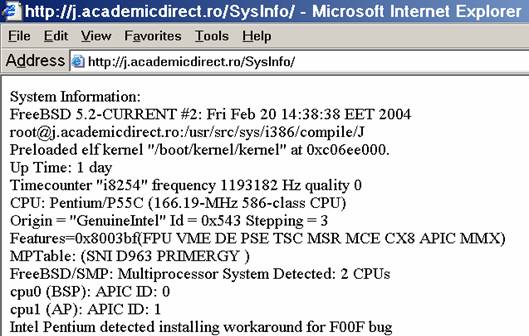
Fig. 1. System type information picture from j.academicdirect.ro server
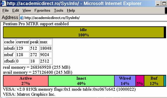
Fig. 2. Memory and CPU usage information picture from ns.academicdirect.ro server
| Filesystem | Size | Used | Avail | Capacity | iused | ifree | %iused | Mounted
|
| /dev/ad0s1a | 35G | 2.5G | 30G | 8% | 194.2K | 4.4M | 4% | /
|
| devfs | 1.0K | 1.0K | 0B | 100% | 0 | 0 | 100% | /dev
|
| procfs | 4.0K | 4.0K | 0B | 100% | 1 | 0 | 100% | /proc
|
| /dev/ad0s1b | 1024M | 0B | 1024M | 0% | 0 | 0 | 100% | none
|
Fig. 3. File system information table from vl.academicdirect.ro server
| Name | Mtu | Network | Address | Ipkts | Ierrs | Opkts | Oerrs | Coll
|
| dc0 | 1500 | (Link#1) | 00:02:e3:08:68:69 | 13612 | 0 | 13883 | 0 | 0
|
| dc0 | 1500 | 172.27.211/24 | 172.27.211.1 | 10716 | - | 15639 | - | -
|
| dc0 | 1500 | 192.168.211 | 192.168.211.1 | 2310 | - | 2424 | - | -
|
| fxp0 | 1500 | (Link#2) | 00:90:27:a5:61:dd | 1017065 | 0 | 729087 | 0 | 0
|
| fxp0 | 1500 | 193.226.7.128 | ns | 78368 | - | 48776 | - | -
|
| lo0 | 16384 | (Link#3) | | 11182 | 0 | 11182 | 0 | 0
|
| lo0 | 16384 | your-net | localhost | 120 | - | 120 | - | -
|
| ppp0* | 1500 | (Link#4) | | 10056 | 1 | 12317 | 0 | 0
|
Fig. 4. Network status information table from ns.academicdirect.ro server
A Performance Counter Application
The second application was used as performance counter. It has also a web interface:
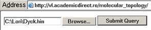
| <form method='post' action='hin.php' enctype='multipart/form-data'>
<input type='file' name='file'>
<input type='submit'>
</form>
|
Fig. 5. Submit form for the hin.php application
About application exploiting experience: there is a bug in Microsoft Internet Explorer 4.01 that does not allow header incomings for downloading of the output file. There is no paper devoted to this subject, in our best knowledge. There is also a bug in Microsoft Internet Explorer 5.5 that interferes with this, which can be solved by upgrading to Service Pack 2 or later. Anyway, this problem does not affect our program. The output data of execution for all three servers is presented in table 1:
Table 1. Statistics of the hin.php Program Execution
| ip | name | CPU | RAM | mics (start) | s. (start) | mics (stop) | s. (stop) | time (s)
|
| 140 | j | 2P166MMX | 128 | 0.565873 | 1077348916 | 0.213418 | 1077349252 | 335.6475
|
| 211 | ns | P2/400 | 256 | 0.634248 | 1077349090 | 0.432039 | 1077349225 | 134.7978
|
| 200 | vl | P3/800 | 512 | 0.623252 | 1077305562 | 0.632815 | 1077305616 | 54.00956
|
The data from table 1 allow us to put on a chart the compared results. An observation is immediate: the time-time dependence from one generation to another one of Pentiums is almost linear, considering only the usage of pointer, string, and integer instructions (without any floating point instructions). In terms of performance, it means just a speed meter. Also, note that: the usage of dual processor system is not different from the single processor one. A possible explanation comes from the algorithm design, which is classical, not a parallel one.
Fig. 6. Execution time vs. 1/CPU frequency
About deviation from linear dependence (Fig. 6 - all lines are draws from 0): it appears that the same real time for the processor is used more efficiently for instructions processing in P II processors in comparison to the P processors and the jump is more obviously at P III architectures.
Dial-In Service
The system preparation can start from kernel configuration. Putting a line like:
options CONSPEED=115200
the kernel will use the serial port as default at 115200 bps (instead of 9600 bps) and of course, the kernel must be recompiled. Anyway, looking at kernel boot messages, we must check if the sio device is installed on the system and is working (dmesg | grep sio). The /etc/ttys file specifies various information about terminals on the system, including about sio ports. Usually a program gets the control of sio port at the boot time. We chouse do not use the default program for sio console (getty), because this do not control correctly the modem, and we use the mgetty program [[16]. Therefore, our entry lines in /etc/ttys file for sio port (called ttyd on FreeBSD system) are like:
ttyd0 "/usr/local/sbin/mgetty -s 115200" dialup on secure
The mgetty program has advantage to control also fax incomings (if the modem support this feature, at least class 2.0 fax). At the end of the mgetty program, we must create the configuration file (/usr/local/etc/mgetty+sendfax/mgetty.config):
direct NO
blocking NO
port-owner uucp
port-group uucp
port-mode 0660
toggle-dtr YES
toggle-dtr-waittime 500
data-only NO
fax-only NO
modem-type auto
init-chat "" ATS0=0Q0&D3&C1 OK
modem-check-time 3600
rings 3
answer-chat "" ATA CONNECT \c \r
answer-chat-timeout 30
autobauding NO
ringback NO
ringback-time 30
ignore-carrier false
issue-file /etc/issue
prompt-waittime 500
login-prompt @!login:
login-time 3600
diskspace 102400
notify lori
fax-owner uucp
fax-group modem
fax-mode 0660
For incoming calls receiving, the /usr/local/etc/mgetty+sendfax/dialin.config file must contain allowed incoming calls (all). The squid service must be installed in the system and must be proper configured:
acl ppp src 192.168.211.0/24
assuming that our dial-in intranet network will use 192.168.211.XXX address class. To transfer the packets to a network card, the /etc/rc.conf file must contain an alias:
ifconfig_dc0_alias0="inet 192.168.211.1 netmask 255.255.255.0"
or the gateway service to be enabled:
gateway_enable="YES"
If the ppp and tun devices are compiled into kernel, a good idea is to disable the module loadings to avoid over configurations (/boot/loader.conf file):
if_tun_load="NO"
if_ppp_load="NO"
For ppp service two utilities are available on a FreeBSD system: ppp and pppd. The ppp service uses the tun device and the pppd service use the ppp device. The used service it can be specified into /usr/local/etc/mgetty+sendfax/login.config file.
Using of ppp Service (tun Device)
The /usr/local/etc/mgetty+sendfax/login.config file it must contain a line like:
/AutoPPP/ - - /etc/ppp/ppp-dial
which will start automatically the ppp service using /etc/ppp/ppp-dial shell script. Not that the /etc/ppp/ppp-dial file must have execution bit set:
-rwxr-xr-x 1 root wheel 45 Feb 3 15:19 /etc/ppp/ppp-dial
(ls al command) therefore, a
chmod +x /etc/ppp/ppp-dial
command will solve the problem. The /etc/ppp/ppp-dial shell script must launch the ppp daemon in direct mode:
#!/bin/sh exec /usr/sbin/ppp direct server
The ppp daemon will start using the /etc/ppp/ppp.conf configuration file. Note that the spaces from the beginning of rows are relevant here:
server:
 set dial "ABORT BUSY ABORT NO\\sCARRIER TIMEOUT 5 \"\" AT \
 OK-AT-OK ATE1Q0 OK \\dATDT\\T TIMEOUT 40 CONNECT"
 set ifaddr 192.168.211.1 192.168.211.2-192.168.211.3
 enable pap proxy passwdauth
 accept dns
Normally, the receiver of a connection requires that the peer authenticate itself. This may be done using login, but alternatively, you can use PAP (Password Authentication Protocol) or CHAP (Challenge Handshake Authentication Protocol). CHAP is the more secure of the two, but some clients may not support it. Our script (see above) use pap method. Anyway, ppp daemon looks for /etc/ppp/ppp.secret file in order to authenticate the client. This file contains one line per possible client, each line containing up to five fields. As example, our configuration file it contains:
lori lori * lori *
All must be ok for the ppp daemon with these configurations. Note that a good idea is to protect our /etc/ppp/ppp.secret file:
chmod 0400 /etc/ppp/ppp.secret
Using of pppd Service (ppp Device)
The /usr/local/etc/mgetty+sendfax/login.config file it must contain a line like:
/AutoPPP/ - - /etc/ppp/pppd-dial
which will start automatically the pppd service using /etc/ppp/pppd-dial shell script. Not that the /etc/ppp/ppp-dial file must have execution bit set:
-rwxr-xr-x 1 root wheel 171 Feb 3 18:12 /etc/ppp/pppd-dial
(ls al command) therefore, a
chmod +x /etc/ppp/pppd-dial
command will solve the problem. The /etc/ppp/pppd-dial shell script must launch the pppd daemon. Note that the pppd daemon does not use the configuration from ppp.conf file, and therefore the configuration must be gives here:
#!/bin/sh exec /usr/sbin/pppd auth 192.168.211.1:192.168.211.2 192.168.211.1:192.168.211.3
	nodefaultroute ms-dns 193.226.7.211 ms-wins 193.226.7.211 ms-wins 172.27.211.2
At present, pppd supports two authentication protocols: PAP and CHAP. PAP involves the client sending its name and a clear text password to the server to authenticate it. In contrast, the server initiates the CHAP authentication exchange by sending a challenge to the client (the challenge packet includes the server's name). The client must respond with a response which includes its name and a hash value derived from the shared secret and the challenge, in order to prove that it knows the secret. The PPP device, being symmetrical, allows both peers to require the other to authenticate itself. In that case, two separate and independent authentication exchanges will occur. The two exchanges could use different authentication protocols, and in principle, different names could be used in the two exchanges. The default behavior of pppd is to agree to authenticate if requested, and to not require authentication from the peer. However, pppd will not agree to authenticate itself with a particular protocol if it has no secrets, which could be used to do so. Pppd stores secrets for use in authentication in secrets files (/etc/ppp/pap-secrets for PAP, /etc/ppp/chap-secrets for CHAP). Both secrets files have the same format. The secrets files can contain secrets for pppd to use in authenticating itself to other systems, as well as secrets for pppd to use when authenticating other systems to it. Each line in a secrets file contains one secret. A given secret is specific to a particular combination of client and server - that client to authenticate it to that server can only use it. Thus, each line in a secrets file has at least three fields:
the name of the client,
the name of the server, and
the secret.
These fields may be followed by a list of the IP addresses that the specified client may use when connecting to the specified server. Therefore, our PAP/CHAP configuration files contain same secrets:
lori academicdirect.ro lori *
The pppd secret files can have also read protection, like for ppp service:
chmod 0400 /etc/ppp/chap-secrets
chmod 0400 /etc/ppp/pap-secrets
Testing of ppp and tun Devices
The debugging mode of the service allows us to look at the communication history for a connection, to identify configuration mistakes and so on. The default logs file for ppp service is /var/log/ppp.log. After the finishing of configuration process, a good idea is to disable the loggings (set log Phase tun command). Starting with ppp service discussion, another observation is important there: if we are using a windows system for connect to dial-in server, a option must be disabled in windows ppp service configuration: Start/Settings/Dial-Up Networking/lori(connection)/Properties/Security(Advanced security options:)/Require encrypted password - must be UNSET The server message for a debugging mode connection using ppp service is listed there:
Feb 3 17:54:34 ns ppp[647]: Phase: Using interface: tun0
Feb 3 17:54:34 ns ppp[647]: Phase: deflink: Created in closed state
Feb 3 17:54:34 ns ppp[647]: tun0: Command:
	server: set dial ABORT BUSY ABORT NO\sCARRIER TIMEOUT 5 ""
	AT OK-AT-OK ATE1Q0 OK \dATDT\T TIMEOUT 40 CONNECT
Feb 3 17:54:34 ns ppp[647]: tun0: Command:
	server: set ifaddr 192.168.211.1 192.168.211.2-192.168.211.3
Feb 3 17:54:34 ns ppp[647]: tun0: Command:
	server: enable pap proxy passwdauth
Feb 3 17:54:34 ns ppp[647]: tun0: Command:
	server: accept dns
Feb 3 17:54:34 ns ppp[647]: tun0: Phase:
	PPP Started (direct mode).
Feb 3 17:54:34 ns ppp[647]: tun0: Phase:
	bundle: Establish
Feb 3 17:54:34 ns ppp[647]: tun0: Phase:
	deflink: closed -> opening
Feb 3 17:54:34 ns ppp[647]: tun0: Phase:
	deflink: Connected!
Feb 3 17:54:34 ns ppp[647]: tun0: Phase:
	deflink: opening -> carrier
Feb 3 17:54:35 ns ppp[647]: tun0: Phase:
	deflink: /dev/ttyd0: CD detected
Feb 3 17:54:35 ns ppp[647]: tun0: Phase:
	deflink: carrier -> lcp
Feb 3 17:54:39 ns ppp[647]: tun0: Phase:
	bundle: Authenticate
Feb 3 17:54:39 ns ppp[647]: tun0: Phase:
	deflink: his = none, mine = PAP
Feb 3 17:54:39 ns ppp[647]: tun0: Phase:
	Pap Input: REQUEST (lori)
Feb 3 17:54:39 ns ppp[647]: tun0: Phase:
	Pap Output: SUCCESS
Feb 3 17:54:39 ns ppp[647]: tun0: Phase:
	deflink: lcp -> open
Feb 3 17:54:39 ns ppp[647]: tun0: Phase:
	bundle: Network
Feb 3 17:54:50 ns ppp[647]: tun0: Phase:
	deflink: open -> lcp
Feb 3 17:54:50 ns ppp[647]: tun0: Phase:
	bundle: Terminate
Feb 3 17:54:52 ns ppp[647]: tun0: Phase:
	deflink: Carrier lost
Feb 3 17:54:52 ns ppp[647]: tun0: Phase:
	deflink: Disconnected!
Feb 3 17:54:52 ns ppp[647]: tun0: Phase:
	deflink: Connect time: 18 secs: 2177 octets in, 14535 octets out
Feb 3 17:54:52 ns ppp[647]: tun0: Phase:
	deflink: 69 packets in, 47 packets out
Feb 3 17:54:52 ns ppp[647]: tun0: Phase:
	total 928 bytes/sec, peak 3171 bytes/sec on Tue Feb 3 17:54:48 2004
Feb 3 17:54:52 ns ppp[655]: tun0: Phase:
	deflink: lcp -> closed
Feb 3 17:54:52 ns ppp[655]: tun0: Phase:
	bundle: Dead
Feb 3 17:54:52 ns ppp[655]: tun0: Phase:
	PPP Terminated (normal).
The pppd service doesnt have a default file for logging, so we must create it and specify the debugging level in our /etc/ppp/pppd-dial shell script. After the finishing of configuration process, a good idea is to disable the loggings:
Feb 3 17:56:47 ns pppd[656]: pppd 2.3.5 started by root, uid 0
Feb 3 17:56:47 ns pppd[656]: Using interface ppp0
Feb 3 17:56:47 ns pppd[656]: Connect: ppp0 <--> /dev/ttyd0
Feb 3 17:56:50 ns pppd[656]: sent [CHAP Challenge id=0x1
	<1e9195c5294cb50b80401cd9e34f15a89b2b823509 aef6fead7549f8b0ae5695a7710a966996>,
	name = "ns.academicdirect.ro"]
Feb 3 17:56:50 ns pppd[656]: rcvd [CHAP Response id=0x1
	<8126c29e65530d6114658931eaa57390>, name ="lori"]
Feb 3 17:56:50 ns pppd[656]: sent [CHAP Success id=0x1 "Welcome to ns.academicdirect.ro."]
Feb 3 17:56:50 ns pppd[656]: sent [IPCP ConfReq id=0x1
	<addr 192.168.211.1> <compress VJ 0f 01>]
Feb 3 17:56:50 ns pppd[656]: CHAP peer authentication succeeded for lori
Feb 3 17:56:50 ns pppd[656]: rcvd [IPCP ConfReq id=0x1 <compress VJ 0f 01>
	<addr 192.168.211.3> <ms-dns 0.0.0.0> <ms-wins 0.0.0.0> <ms-dns 0.0.0.0> <ms-wins 0.0.0.0>]
Feb 3 17:56:50 ns pppd[656]: sent [IPCP ConfNak id=0x1 <ms-dns 193.226.7.211>
	<ms-wins 193.226.7.211> <ms-dns 193.226.7.211> <ms-wins 172.27.211.2>]
Feb 3 17:56:50 ns pppd[656]: rcvd [IPCP ConfAck id=0x1
	<addr 192.168.211.1> <compress VJ 0f 01>]
Feb 3 17:56:51 ns pppd[656]: rcvd [IPCP ConfReq id=0x2 <compress VJ 0f 01>
	<addr 192.168.211.3> <ms-dns 193.226.7.211> <ms-wins 193.226.7.211>
	<ms-dns 193.226.7.211> <ms-wins 172.27.211.2>]
Feb 3 17:56:51 ns pppd[656]: sent [IPCP ConfAck id=0x2 <compress VJ 0f 01>
	<addr 192.168.211.3> <ms-dns 193.226.7.211> <ms-wins 193.226.7.211>
	<ms-dns 193.226.7.211> <ms-wins 172.27.211.2>]
Feb 3 17:56:51 ns pppd[656]: local IP address 192.168.211.1
Feb 3 17:56:51 ns pppd[656]: remote IP address 192.168.211.3
Feb 3 17:56:51 ns pppd[656]: Compression disabled by peer.
Feb 3 17:57:04 ns pppd[656]: Hangup (SIGHUP)
Feb 3 17:57:04 ns pppd[656]: Modem hangup, connected for 1 minutes
Feb 3 17:57:04 ns pppd[656]: Connection terminated, connected for 1 minutes
Feb 3 17:57:05 ns pppd[656]: Exit.
The ppp and tun devices can be monitored via a web interface. Our results are depicted in table 1:
Table 1. Network status table from ns.academicdirect.ro server
| Name | Mtu | Network | Address | Ipkts | Ierrs | Opkts | Oerrs | Coll
|
| ... | ... | ... | ... | ... | ... | ... | ... | ...
|
| ppp0* | 1500 | (Link#4) | | 18922 | 1 | 23447 | 0 | 0
|
| tun0* | 1500 | (Link#5) | | 9322 | 34 | 12425 | 38 | 0
|
Conclusions
Because the FreeBSD is available free of charge (for individuals and for organizations) to use and comes with full source code, anyone which want a featured server operating system (opposing to NetBSD, a very conservative legal copyright ported software system, or OpenBSD, a very conservative ported software security system) can install it. FreeBSD operating system procedure is easy to follow even if the administrator does not have experience with BSD-like systems.
The feature of boot floppies allows us to install FreeBSD even if we do not have a FreeBSD CD or CD-drive in the system. CVSup mechanism offers an efficient way to maintain and update the system. The kernel recompilation allows us to improve the performance of the system, in terms of speed and memory management. Looking at hardware characteristics and including corresponding options in kernel are obtained a better exploiting of the hardware resources. More, some specific hardware are then detected and configured for use. Creating a backup copy of the kernel, we can undo any action of kernel reinstalling.
If some service does not start automatically, from unknown reasons (such as ftpd on j.academicdirect.ro server), we can try to start manually and after that we can create a script for auto start. Another exemplified situation show that not always the installation scripts puts all required data in configuration files (AddType application/x-httpd-php .php) and if a module does not start, a good idea is to look carefully at service configuration file.
The SysInfo application for system information allows one to inspect the system state via web. The application is useful for system administrators and presumes identification of system failures. The use of the system utilities to obtain the displayed information makes the application portable onto different systems and architectures.
The PHP language offers a very good interface with system utilities and an efficient way to develop client-server applications.
The second application which tests both PHP capabilities and system performance, proves that, even if the constant controlling the number of consecutive calls of recv() recursive function has big values (like 40 or 50), the program does not crash. The comparative study on the three Intel-based systems showed the qualitative difference among various Pentium processor architectures. Surprisingly (or not), using a dual processor system within an interactive time-sharing operating system does not mean that the system makes parallel processing.
The CHAP81 variant of Microsoft Windows operating system creates some misunderstandings in authentication using ppp service (tun device) and only PAP authentication protocol are agreed by the server. The pppd works fine with CHAP81. Same observation is noted for password encryption (see text). The default program for sio device (getty) doesnt offer the full support for modem control, and mgetty program is a good replacement. Kernel recompilation allows us to modify the default communication speed for sio ports. The debugging mode log files is the best starting point if something goes wrong and the communication fails.
References
[1]. UNIX-like operating system official http sites:
debian.org (Debian),
www.linux.org (Linux),
lindows.com (LinwowsOS),
ibm.com/servers/aix/os (AIX),
www.gnu.org (GNU),
hp.com/products1/unix/operating (HP-UX),
opengroup.org (OSF),
sun.com/software/solaris (Solaris),
www.bsd.org (BSD/OS),
netbsd.org (NetBSD),
openbsd.org (OpenBSD),
freebsd.org (FreeBSD),
www.trustedbsd.org (TrustedBSD),
picobsd.org (PicoBSD)
[2]. http://www.bartleby.com/61, The American Heritage Dictionary of the English Language, Fourth Edition.
[3]. http://www.delorie.com/gnu/docs/vera, Virtual Entity of Relevant Acronyms, The Free Software Foundation.
[4]. http://www.instantweb.com/d/dictionary, Free Online Dictionary of Computing.
[5]. www.freebsd.org/cgi/man.cgi, FreeBSD Hypertext Man Pages.
[6]. www.php.net, The PHP Group (Arntzen T. C., Bakken S., Caraveo S., Gutmans A., Lerdorf R., Ruby S., Schumann S., Suraski Z., Winstead J., Zmievski A.).
[7]. http://phpsysinfo.sourceforge.net, Open Source Development Network.
[8]. John D. Polstra, http://www.cvsup.org/faq.html, CVSup Frequently Asked Questions.
[9]. Jäntschi L., Zaharieva-Stoyanova E., Upload a File to a Server. Case Study, UNITECH'03 International Scientific Conference, November 21-22 2003, Gabrovo, Bulgaria, volume I "ISC UNITECH'03 GABROVO Proceedings", p. 274-276.
[10]. Greer D. J., http://www.robelle.com/library/papers/www-paper/clients.html, Dial-in Access, Robelle Solutions Technology Inc.
[11]. http://www.speedtouchdsl.com/supfaq.htm, SpeedTouch DSL modems, Thomson.
[12]. http://www.greatware.net/modems, Modems, Great Internet Software.
[13]. http://server.rotld.ro/cgi-bin/whois?whois=academicdirect.ro, Romanian National R&D Computer Network.
[14]. http://www.apache.org, The Apache Software Foundation.
[15]. http://www.mysql.org, MySQL AB.
[16]. http://www.webforum.de/mgetty-faq.html, Smart Modem Getty, Gert Doering.
Issue 03, p. 031-044
Simulation and Computer Modelling of Carbonate Concentration in Brewery Effluent
O. D. ADENIYI
Department of Chemical Engineering, Federal University of Technology, Minna, Nigeria
Email: lekanadeniyi2002@yahoo.co.uk
Abstract
The development of a mathematical model to predict the concentration of carbonates in effluent discharged from a brewery industry is the aim of this paper. This was achieved by obtaining effluent data for several years and using the method of least squares to develop the model. A mean deviation of 9% was observed by comparing the experimental data with the simulated results. The constituent parameter with the greatest influence on the simulated model was found to be sodium ion (Na+) with a coefficient of 0.87642 while that with the least effect was the temperature with a coefficient of 0.0514255. In addition, a control model was developed to monitor the conversions of the effluent constituents in three Continuous Stirred Tank Reactors (CSTRs), some deviation was observed between the set-point values and the empirical values.
Keywords
Effluent, BOD, pH, brewery, ions, carbonate, model, simulation
Introduction
Recently, much attention has been focused on the development of accurate equations of state for the prediction of several process parameters. Much effort has also been applied to the development of several equilibrium calculation algorithms for handling some numerical complexities that are inherent in the modeling of waste systems. Computing power, data acquisition, simulation, optimization and information systems have greatly improved effluent management over the recent years. To maintain set discharge standards, to the environment, it is imperative to adopt the most efficient effluent monitoring and management system available. In general, the optimization does not represent a radical change in operating procedures to maintain a safe discharge standard. Effluent monitoring systems provide accurate cause and effect relationships of a process. Obtained set point data are used by engineers as analytical tools to understand and improve the process (Luyben, 1995; Richardson and Peacock, 1994; Meyer, 1992a,b,c; Austin, 1984).
In Nigeria, the last two decades have marked the emergence of several indigenous and foreign breweries. The high demand for brewery products, as well as the technological advancement in this regards, have further accelerated the growth of this industries. In Nigeria, there are nineteen breweries, and the waste generated is one of the major sources of industrial waste hazards. Improper handling and disposal could easily constitute a problem to both the people and the environment. The solid waste could be a source and reservoir to epidemic disease such as cholera and typhoid fever. The liquid effluent, though less noticeable as a waste, constitutes more hazard than the easily noticeable solid waste. The liquid effluent, on percolation into shallow wells could be a direct source of contamination to portable water. When this reached into streams, the danger to public health is as a result of the consumption of polluted water by the unsuspecting public, the aquatic as well as the land animals. Polluted water could lead to the migration of fishes from streams and rivers or outright death of the fishes. The surviving ones may become sick and unpalatable, the result of which may have an economic impact on the surrounding communities. Even when aquatic life survives in the polluted stream, it is not a proof of pollution free environment as some aquatic animals such as shell-fish have been noticed to survive and even thrive in polluted waters. Some chemical constituents of brewery waste (e.g. Chromium) could be accumulated by plants and from there, enter the food chain and be consumed by humans, this could enhance the development of some terminal disease such as cancer (Eckenfelder, 1989; Nikoladze et-al, 1989; Welson and Wenetow, 1982; Suess, 1982; Kriton, 1980).
For brewery effluent, the prevailing pH value is the resultant of the disassociation of organic and inorganic compounds and their subsequent parameters are in principle targeted at measuring characteristics that could evaluate the extent or possibility of disassociation of organic or inorganic compounds and their subsequent hydrolysis. In other words measured but are not additive functions. Effluents form breweries can be characterized based on the relative oxygen demand, expressed as biochemical oxygen demand (BOD) or chemical oxygen demand COD, suspended solids (SS), pH, Temperature and flow parameters (Odigure and Adeniyi, 2002; Luyben, 1995; Imre 1984, Suess 1982).
The aim of this paper is to develop a model equation to predict the concentration of carbonate ions (CO32-) in brewery effluent, this would be achieved by utilizing, computer simulation techniques. In addition the paper seeks to monitor and control the concentration of CO32- in 3 CSTRs connected in series.
Conceptualization and Model Development
In the effluent stream, the components of consideration are
Cl-, CO32-, Na+, Ca2+
Na+ + Cl- → NaCl (1)
Ca2+ + CO32- → CaCO3 (2)
The liquid effluent from the brewery is charged into a series of 3 CSTR, where product B is produced and reaction A is consumed according to the first order reaction, occurring in the fluid. The feed back controller used for this system, is a Proportional and Integral controller (PI). The controller looks at the product concentration leaving the third tank (CA3) and makes adjustments in the inlet concentration to the first reaction CA0 in order to keep CA3 near its desired set point value CA3set (Levenspiel, 1997; Fogler, 1997; Luyben, 1995; Richardson and Peacock, 1994; Smith, 1981).
The variable CAD is the disturbance concentration, and the variable CAM is the manipulated concentration that is changed by the controller. From the system, it can be postulated that:
CA0 = CAM + CAD (3)
The controller has proportional and integral action; it changes CAM, based on the magnitude of the error (the difference between the set point concentration and CA3) and the integral of this error.
CAM = 0.8 + Kc(E + 1/דf∫E(t)dt ) (4)
where:
E = CA3set - CA3 (5)
Kc = Feed back Controller gain
Ίf = Feed back Controller space- time constant (minutes).
The 0.8 term is the bias value of the controller, that is, the value of CAM at time equal zero. Numerical values of Kc = 30, דf = 5 minutes are used (Perry and Green, 1997; Luyben, 1995; Himmelblau, 1987; Imre, 1986).
The industrial brewery effluent, has the following measured parameters; potency of hydrogen (pH), temperature (TEMP), total dissolved solid (TDS), biochemical oxygen demand (BOD), carbonate ions (CO32-), calcium ions (Ca2+), sodium ions (Na+) and chloride ions (Cl -).
Let pH =P, Temp = T1, TDS = T2, BOD = B, CO32- = C, Ca = C1, Na = N, Cl = C2
To develop a model for the concentration of CO32- ion as a function of the other parameters in the effluent we have:
C = f (P, T1, T2, B, C1, N, C2) = f (aP, bT1, cT2, dB, eC1, f N, gC2) (6)
where C is the dependent variable, a, b, c, d, e, f and g are the coefficients, which should be determined, while P, T1, T2, B C1, N, C2 are the independent variables of the equation.
To develop the model the linear regression techniques (least square method) was applied (Stroud, 1995a,b; Carnahan et-al, 1969). Let Z represent the square of the error, between the observed value and the predicted value. Mathematically:
Z = Observed value (aP + bT1 + cT2 + dB + eC1 + fN + gC2)2 (7)
For n experimental values of P, T1, T2, B, C1, N, C2 we have:
nZ = Σ (Vi (aPi + bT1i + CT2i + dBi + eC1i + fNi + gC2i)2 (8)
We could minimize the error of this regression, by finding the derivative of nZ with respect to the constant a, b, c, d, e, f, g and equating to zero.
∂(nz)/∂a = -2∑Pi(Vi(aPi+bT1i+cT2i+dBi+eC1i+fNi+gC2i)) = 0
∂(nz)/∂b = -2∑T1i(Vi(aPi+bT1i+cT2i+dBi+eC2i+fNi+gC2i)) = 0
∂(nz)/∂c = -2∑T2i(Vi(aPi+bT2i+cT2i+dBi+eC1i+fNi+gC2i)) = 0
∂(nz)/∂d = -2∑Bi(Vi (aPi+bT1i+cT2i+dBi+eC1i+fNi+gC2i)) = 0 (9)
∂(nz)/∂e = -2∑Ci(Vi(aPi+bT2i+cT2i+dBi+eC1i+fNi+gC2i)) = 0
∂(nz)/∂f = -2∑Ni(Vi(aPi+bT1i+CT2i+dBi+eC1i+fNi+gC2i)) = 0
∂(nz)/∂g = -2∑C2i(Vi(aPi+bT1i+CT2i+dBi+eC1i+fNi+gC2i)) = 0
Dividing both sides by 2 and rearranging, we obtain:
∑PiVi=a∑ pi2+b∑ TiPi+c∑T2iPi+d∑BiPi+e∑CiPi+f∑NiPi+g∑C2iPi
∑T1iVi=a∑piTi+b∑Tii2+c∑T2iT1i+d∑BiT1i+e∑C1iT1i+f∑NiT1i+g∑C2iT1i
∑T2Vi=a∑piT2i+b∑TiiT2i+c∑T2i2+d∑BiT2i+e∑C1iT2i+f∑NiT2i+g∑C2iT2i
∑BiVi=a∑PiBi+b∑T1iBi+c∑T2iBi+d∑Bi2+e∑C1iBi+f∑NiBi+g∑C2iBi (10)
∑C1iVi=a∑PiC1i+b∑T1iC1i+c∑T2iC1i+d∑BiC1i+e∑C1i2+f∑NiC1i+g∑C2iC1i
∑NiVi=a∑PiNi+b∑T1iNi+c∑T2iNi+d∑BiNi+e∑C1iNi+f∑Ni2+g∑C2iNi
∑C2iVi=a∑PiC2i+b∑T1iC2i+c∑T2iC2i+d∑BiC2i+e∑C1iC2i+f∑NiC2i+g∑C2i2
The following values were obtained from mathematical calculation (Stroud, 1995a,b; Carnahan et-al, 1969):
∑P12 = 12276.64∙108; ∑Pi Ti = 2845.59∙104; ∑T2iPi = 930.88∙104;
∑BiPi = 0.254900000; ∑C1iPi = 928.8557∙104; ∑Ni Pi = 841.99000∙104;
∑C2iPi = 174.6000∙104; ∑PiT1i = 2845.59∙104; ∑Ti2=94740.84∙104;
∑T2iT1i = 2377.36∙104; ∑BiTi = 0.708970000000; ∑CiT1i = 2641.97∙104;
∑NiTi = 2340.830∙104; ∑C2iT1i = 441.74∙104; ∑C1iT2 = 845.600000∙104;
∑NiT2i = 760.7∙104; ∑C2iT2i =157.500000∙10-4; ∑C1iBi = 0.23145000; (11)
∑NiBi = 0.20413000000; ∑C2iBi = 39.34∙10-3; ∑NiC1i = 764.2002∙10-4;
∑C2iC1i = 156.458∙10-4; ∑C2iNi = 142.9500∙10-4; ∑Ti2 = 10179.2∙108;
∑T1i2 = 94740.84∙10-4; ∑Bi2 = 762.864∙106; ∑Ci2 = 10124.38∙10-8;
∑Ni2 = 7144.814∙108; ∑C2i2 = 351.7600∙10-8; ∑PiVI = 924.2800∙10-4;
∑T1iVi = 2568.1∙104; ∑T2iVi = 839.400∙10-4; ∑BiVi = 0.2297000;
∑C1iVi = 838.86∙10-4; ∑NiVi = 763.3∙104; ∑C2iVi = 156.33∙10-4.
Substituting the values obtained into the equation, we have:
a(12276.64∙10-8) + b(2845.59∙10-4) + c(930.88∙10-4) + d(0.2549)
+ e(928.86∙10-4) + f(841.99∙10-4) + g(174.60∙10-4) = 924.28∙104
a(2845.59∙10-8) + b(94740.84∙10-8) + c(2377.74∙10-4) + d(0.709)
+ e(2641.97∙10-4) + f(2340.83∙10-4) + g(441.74∙10-4) = 2568.1∙104
a(930.88∙10-4) + b(2377.36∙10-4) + c(10179.2∙10-8) + d(0.2326)
+ e(845.6∙10-4) + f(760∙10-4) + g (157.5∙10-4) = 839.4∙104 (12)
a(0.2549) + b(0.709) + c(0.2326) + d(762.864∙10-6)
+ e (0.23145) + f(0.20413) + g (39.34 10-3) = 0.2297
a(928.86∙10-4) + b(2621.97∙10-4) + c(845.6∙10-4) + d(0.23145)
+ e(10124.38∙10-8) + f(764.202∙104) + g(156.458∙10- 4) = 838.86∙104
a(841.99∙10-4) + b(2340.83∙10-4) + c(760.7∙10-4) + d(0.20413)
+ e(764.202∙10-4) + f(7144.814∙10-8 ) + g(142.95∙10-4) = 763.3∙104
a(174.60∙10-4) + b(441.74∙10-4) + c(157.5∙10-4) + d(39.34∙10-3)
+ e(156.458∙10-4) + f(142.95∙10-4) + g (351.76∙10-8) = 156.33∙104
A computer program, coded in C++ was developed to solve the 7´7 matrices and the resulting model is:
C = 0.163488P + 0.0514255T1 + 0.166722T2 + 0.0596487B
+ 0.182077C1 + 0.87642N + 0.821217C2 (13)
Results and Discussion
The effluent from the brewery was discharged at different points such as the tank cellars, bottling hall, brew house and filter-room. The effluent analyzed in this study was however obtained from the combined effluent discharge collection point. The analytical results are presented in Tables 1, 2 and 3.
Table 1. Analysis of effluent discharge from brewery industry (1999)
|
|
pH
|
TEMP
(°C)
|
TDS
(kg/dm3)
|
BOD
(kg/dm3)
|
CO32-
(kg/dm3)
|
Ca2+
(kg/dm3)
|
Na+
(kg/dm3)
|
Cl-
(kg/dm3)
|
|
Jan
|
9.60
|
27.60
|
8.211
|
2.35∙10-3
|
13.8421
|
8.480
|
8.106
|
1.477
|
|
Feb
|
9.00
|
28.20
|
8.120
|
2.30∙10-3
|
13.6687
|
8.146
|
8.125
|
1.523
|
|
Mar
|
9.50
|
26.50
|
8.000
|
2.35∙10-3
|
14.9868
|
8.742
|
8.636
|
1.612
|
|
Apr
|
9.20
|
26.00
|
9.512
|
2.40∙10-3
|
14.8273
|
8.102
|
8.064
|
1.585
|
|
May
|
9.30
|
26.00
|
8.167
|
2.30∙10-3
|
13.9182
|
8.261
|
8.093
|
1.532
|
|
Jun
|
9.40
|
24.50
|
8.000
|
2.00∙10-3
|
13.7231
|
7.992
|
7.602
|
1.632
|
|
Jul
|
9.40
|
26.00
|
8.261
|
2.30∙10-3
|
13.5698
|
8.266
|
8.611
|
1.723
|
|
Aug
|
9.10
|
26.50
|
8.082
|
2.35∙10-3
|
14.8955
|
8.361
|
8.626
|
1.439
|
|
Sep
|
9.00
|
24.00
|
8.664
|
2.44∙10-3
|
14.0688
|
8.073
|
8.0423
|
1.321
|
|
Oct
|
9.00
|
24.00
|
8.164
|
2.40∙10-3
|
13.5890
|
8.042
|
7.110
|
1.732
|
|
Nov
|
9.20
|
26.00
|
9.026
|
2.40∙10-3
|
13.9936
|
8.364
|
8.210
|
1.521
|
|
Dec
|
9.10
|
24.50
|
8.164
|
2.33∙10-3
|
13.9814
|
8.772
|
8.116
|
1.621
|
The effluent was analyzed based on several parameters of pH, temperature and ionic content (CO32-, TDS, Ca, Na, Cl, BOD). From the empirical results presented on Tables 1 to 3, it was observed that the determinant ion is CO32-, because of its high concentration and its high acidity.
Table 2. Analysis of effluent discharge from brewery industry (2000)
|
|
pH
|
TEMP
(°C)
|
TDS
(kg/dm3)
|
BOD
(kg/dm3)
|
CO32-
(kg/dm3)
|
Ca2+
(kg/dm3)
|
Na+
(kg/dm3)
|
Cl-
(kg/dm3)
|
|
Jan
|
9.40
|
26.50
|
8.575
|
2.37∙10-3
|
13.0842
|
8.183
|
8.105
|
1.532
|
|
Feb
|
9.10
|
26.00
|
8.324
|
2.33∙10-3
|
13.9271
|
8.176
|
8.173
|
1.561
|
|
Mar
|
9.70
|
27.00
|
8.175
|
2.40∙10-3
|
13.9866
|
8.233
|
8.621
|
1.663
|
|
Apr
|
9.30
|
24.00
|
8.025
|
2.30∙10-3
|
13.1182
|
8.136
|
7.189
|
1.419
|
|
May
|
9.10
|
25.00
|
8.000
|
2.36∙10-3
|
13.3970
|
8.491
|
7.326
|
1.567
|
|
Jun
|
9.10
|
28.00
|
8.000
|
2.37∙10-3
|
13.774
|
8.247
|
7.961
|
1.668
|
|
Jul
|
9.20
|
26.30
|
8.232
|
2.40∙10-3
|
13.0736
|
8.566
|
6.119
|
1.589
|
|
Aug
|
9.40
|
24.50
|
8.727
|
2.20∙10-3
|
13.0180
|
8.373
|
6.327
|
1.772
|
|
Sep
|
9.00
|
23.00
|
8.632
|
2.25∙10-3
|
13.0000
|
8.392
|
6.331
|
1.699
|
|
Oct
|
9.30
|
26.00
|
8.442
|
2.40∙10-3
|
13.2941
|
8.626
|
6.861
|
1.427
|
|
Nov
|
9.10
|
28.00
|
8.665
|
2.35∙10-3
|
13.5084
|
8.286
|
7.544
|
1.489
|
|
Dec
|
9.10
|
24.00
|
8.361
|
2.33∙10-3
|
13.5126
|
8.725
|
7.612
|
1.551
|
The data presented are combined effluent discharge data for three different years (1999, 2000, and 2001), in all cases the carbonate ion was observed to dominate in concentration. Therefore part of the aims of this work is to develop appropriate techniques to conveniently reduce the concentration of this ion. The process chosen for this task was characterized by two neutralization reactions occurring simultaneously in the reaction vessel as given by Equation 1 and 2. (Meyer, 1992a,b,c; Luyben, 1990, Austin, 1984).
The principal reactions of consideration are Equation 1, where the model equation is represented as:
A + B → C (14)
where A is Calcium ion; B is Carbonate ion; C is Calcium carbonate.
The limiting reactant is B and its conversion is of interest in this research work. Appropriate software coded in Visual Basic was developed to monitor the concentration of the carbonate ions in the system, the results are presented on Tables 7, 8 and 9. From the Tables it was observed that there was a change in concentration (conversion) across the tanks in series, this change was attributed to the reaction given by Equation 1.
Table 3. Analysis of effluent discharge from brewery industry (2001)
|
|
pH
|
TEMP
(°C)
|
TDS
(kg/dm3)
|
BOD
(kg/dm3)
|
CO32-
(kg/dm3)
|
Ca2+
(kg/dm3)
|
Na+
(kg/dm3)
|
Cl-
(kg/dm3)
|
|
Jan
|
9.70
|
28.00
|
8.164
|
2.30∙10-3
|
13.973
|
8.274
|
7.994
|
1.6114
|
|
Feb
|
8.90
|
28.30
|
8.180
|
2.30∙10-3
|
13.083
|
8.354
|
8.074
|
1.6114
|
|
Mar
|
9.60
|
26.00
|
7.990
|
2.40∙10-3
|
14.886
|
8.399
|
8.883
|
1.7390
|
|
Apr
|
9.10
|
24.00
|
9.410
|
2.44∙10-3
|
12.818
|
7.832
|
6.495
|
1.5650
|
|
May
|
9.30
|
26.40
|
8.082
|
2.36∙10-3
|
12.545
|
8.286
|
6.514
|
1.4450
|
|
Jun
|
9.40
|
24.00
|
7.999
|
1.71∙10-3
|
14.922
|
8.626
|
9.061
|
1.7390
|
|
Jul
|
9.70
|
27.90
|
7.999
|
2.30∙10-3
|
14.367
|
8.399
|
8.291
|
1.5890
|
|
Aug
|
9.00
|
26.40
|
8.263
|
2.35∙10-3
|
13.262
|
8.399
|
8.291
|
1.6114
|
|
Sep
|
8.80
|
22.50
|
9.163
|
2.33∙10-3
|
12.471
|
8.853
|
6.119
|
1.5470
|
|
Oct
|
9.10
|
24.90
|
8.090
|
2.41∙10-3
|
12.584
|
8.286
|
6.514
|
1.5730
|
|
Nov
|
9.30
|
26.30
|
9.412
|
2.37∙10-3
|
12.604
|
8.286
|
6.317
|
1.4320
|
|
Dec
|
8.90
|
23.10
|
8.131
|
2.35∙10-3
|
13897
|
8.626
|
8.488
|
1.2920
|
For the first case the feed enters the first reactor with the following concentrations: CA2 at 10 kg/dm3, CA3 at 0.1 kg/dm3 while CAM is at 0.8 kg/dm3 (which is the bias value of the controller at time zero, T = 0), the feedback controller used for this process has proportional and integral action (PI controller), it changes CAM based on the magnitude of the error. The value of the set point, CA3set was at 0.1 kg/dm3, the controller looks at the product concentration leaving the third Tank, CA3, and makes adjustments in the inlet concentration to the first reactor, CA0, in order to keep CA3 near its set point CA3set. The variable CAD is the disturbance concentration and the variable CAM is the manipulated concentration that was changed by the controller (Equation 3).
For this particular simulation (applying Equations 3 and 4), the following values were used; Kc at 30, דf at 5minutes. Critical observation shows that the output concentration of the system (CA3) approaches the set point concentration (CA3set), as shown Table 7 to 9. The difference between the set point value and CA3 in each case is small, this was attributed to the reactor design specification and reactor operating condition (Luyben, 1990; Himmelblau, 1987). Generally, the whole essence of the process set-up is to neutralize the concentration of the carbonate ions to values low enough, so as not to be toxic to the environment, and to a reasonable extent this was achieved.
Tables 1-3 gives the analysis of the effluent discharge from the brewery industry for three consecutive years.
The pH values for the years are slightly high, with a minimum of 9.00 for the first two years and 8.90 for the third year. On the general the pH were mostly alkaline from the discharge. The temperature was within the set limits by the Federal Environmental Protection Agency (FEPA). The limits of the other parameters were also within the acceptable limits. The facts is that all these compounds present in the effluent could be hydrolyzed by water, that is, the ions of these compounds could be exchanged with water molecules (Odigure and Adeniyi, 2002; Karapetyant and Drakin, 1981). The carbonate ions concentrations from Table 1-3 are relatively higher than the other parameters.
Comparative values for the concentration of carbonate between the empirical and simulation are presented in Tables 4 to 6.
The highest deviation for 1999 was 8.70%, for 2000 was 5.50% and 1.70% for 2001. The deviation of the simulated values from that of the empirical could be attributed to certain limitations placed during model development.
Table 4. Comparative values for empirical and simulation of CO32- (1999)
|
|
Empirical
(kg/dm3)
|
Simulated
(kg/dm3)
|
Deviations
|
%Errors
|
|
Jan
|
13.8421
|
14.2193
|
-0.3772
|
2.73
|
|
Feb
|
13.6687
|
14.1303
|
-0.4616
|
3.38
|
|
Mar
|
14.9868
|
14.6850
|
0.4129
|
2.76
|
|
Apr
|
14.8273
|
14.4144
|
0.4129
|
2.78
|
|
May
|
13.9182
|
14.0744
|
-0.1562
|
1.12
|
|
Jun
|
13.7231
|
13.5885
|
0.1346
|
0.98
|
|
Jul
|
13.5698
|
14.7508
|
-1.181
|
8.70
|
|
Aug
|
14.8955
|
14.4622
|
0.4333
|
2.91
|
|
Sep
|
14.0688
|
13.7540
|
0.3148
|
2.24
|
|
Oct
|
13.5890
|
13.1848
|
0.4042
|
2.97
|
|
Nov
|
13.9936
|
14.3135
|
-0.3199
|
2.29
|
|
Dec
|
13.9814
|
14.1535
|
-0.1689
|
1.21
|
That is, apart from these seven parameters considered there could be other factors, which contributed to the level of carbonates in the effluent. One is the interactions, which the effluents would have undergone during the process of flowing through the discharge path.
Table 5. Comparative values for empirical and simulation of CO32- (2000)
|
|
Empirical
(kg/dm3)
|
Simulated
(kg/dm3)
|
Deviations
|
%Errors
|
|
Jan
|
13.0842
|
12.7240
|
0.3602
|
2.75
|
|
Feb
|
13.9271
|
14.0867
|
-0.1596
|
1.15
|
|
Mar
|
13.9866
|
14.7578
|
-0.7712
|
5.50
|
|
Apr
|
13.1182
|
13.0387
|
0.0795
|
0.60
|
|
May
|
13.3970
|
13.3595
|
0.0375
|
0.30
|
|
Jun
|
13.7740
|
14.1089
|
-0.3349
|
2.40
|
|
Jul
|
13.0736
|
12.4553
|
0.6183
|
4.70
|
|
Aug
|
13.0180
|
12.7754
|
0.2426
|
1.90
|
|
Sep
|
13.0000
|
12.5641
|
0.4359
|
3.40
|
|
Oct
|
13.2941
|
13.0194
|
0.2747
|
2.10
|
|
Nov
|
13.5084
|
13.7144
|
-0.2060
|
1.50
|
|
Dec
|
13.5126
|
13.6484
|
-0.1358
|
1.00
|
Table 6. Comparative values for empirical and simulation of CO32- (2001)
|
|
Empirical
(kg/dm3)
|
Simulated
(kg/dm3)
|
Deviations
|
%Errors
|
|
Jan
|
13.973
|
14.2132
|
-0.2373
|
1.70
|
|
Feb
|
13.083
|
12.9527
|
0.1303
|
1.00
|
|
Mar
|
14.886
|
14.9830
|
-0.097
|
0.65
|
|
Apr
|
12.818
|
12.6945
|
0.1235
|
0.96
|
|
May
|
12.545
|
12.6300
|
-0.085
|
0.68
|
|
Jun
|
14.922
|
15.0447
|
-0.1227
|
0.82
|
|
Jul
|
14.367
|
14.4452
|
-0.0782
|
0.54
|
|
Aug
|
13.262
|
13.3709
|
-0.1089
|
0.82
|
|
Sep
|
12.471
|
12.3688
|
0.1022
|
0.82
|
|
Oct
|
12.584
|
12.6266
|
-0.0426
|
0.34
|
|
Nov
|
12.604
|
12.6633
|
-0.0593
|
0.47
|
|
Dec
|
13.897
|
14.0094
|
-0.1124
|
0.81
|
Consequently, pollutants present in water could seriously affect the resultant carbonate concentration. The extent of acidification or alkalization of the solution by pollutants is dependent, on not only the chemical nature of the compounds present, but also the prevailing technological conditions (Odigure and Adeniyi, 2002). From the calculated coefficients, it could be seen that the carbonate concentration is most affected by the sodium ions and least by the temperature.
Tables 7- 9 gives the time-concentration value from simulation of the months of January, March and June of the year 2001.
Table 7: Time Concentration data from simulation (Jan. 2001)
|
Run
|
Time
(min)
|
CA1
(kg/dm3)
|
CA2
(kg/dm3)
|
CA3
(kg/dm3)
|
CAM
(kg/dm3)
|
|
1
|
0.00
|
13.0830
|
10.0000
|
0.1000
|
0.8000
|
|
2
|
0.50
|
1.7949
|
7.5767
|
1.8086
|
53.3328
|
|
8
|
3.51
|
9.2574
|
1.9208
|
1.6843
|
48.9541
|
|
12
|
5.51
|
1.0135
|
2.9864
|
1.1401
|
32.2791
|
|
19
|
9.01
|
7.1980
|
1.2045
|
0.3007
|
13.1300
|
|
20
|
9.51
|
5.6166
|
2.0257
|
0.1556
|
3.2070
|
From Table 7 at time zero, the conversion of CO32- was 0.8 kg/dm3 (which is the bias value of the controller), at T=0.5 minutes, the conversion was 53.33278 kg/dm3, showing that with increase in time the manipulated variable concentration decreases proportionately toward the set point. The same pattern was observable in Table 8 and 9.
Table 8: Time Concentration data from simulation (Mar. 2001)
|
Run
|
Time
(min.)
|
CA1
(kg/dm3)
|
CA2
(kg/dm3)
|
CA3
(kg/dm3)
|
CAM
(kg/dm3)
|
|
1
|
0.00
|
14.8860
|
10.0000
|
0.1000
|
0.8000
|
|
2
|
0.50
|
2.8012
|
7.8471
|
1.8242
|
54.3856
|
|
8
|
3.51
|
9.1626
|
2.1493
|
1.7621
|
50.7102
|
|
12
|
5.51
|
0.7137
|
3.1506
|
1.1611
|
32.9314
|
|
19
|
9.01
|
7.4191
|
1.1768
|
0.3364
|
14.0958
|
|
20
|
9.51
|
5.9060
|
2.0619
|
0.1355
|
0.5531
|
Table 9: Time Concentration data from simulation (Jun. 2001)
|
Run
|
Time
(min.)
|
CA1
(kg/dm3)
|
CA2
(kg/dm3)
|
CA3
(kg/dm3)
|
CAM
(kg/dm3)
|
|
1
|
0.00
|
14.9220
|
10.0000
|
0.1000
|
0.8000
|
|
2
|
0.50
|
2.8213
|
7.8525
|
1.8431
|
54.4067
|
|
8
|
3.51
|
9.1607
|
2.1539
|
1.7638
|
50.7430
|
|
12
|
5.51
|
0.7078
|
3.1538
|
1.1655
|
32.9445
|
|
19
|
9.01
|
7.4236
|
1.1762
|
0.3371
|
14.1151
|
|
20
|
9.51
|
5.9118
|
2.0626
|
0.1351
|
0.5648
|
Table 10 gives the percentage error deviation analysis of the simulated concentration for the third tank to that of the set point. This gives the deviation error analysis for the process control model. The highest deviation was 38% at the fifth run.
Table 10: Error deviation analysis for process control model
|
Run
|
CA3
|
CA3set
|
Error Deviation
|
% Error Deviation
|
|
1
|
0.14565
|
0.1
|
0.04565
|
31
|
|
2
|
0.15564
|
0.1
|
0.05560
|
36
|
|
3
|
0.13548
|
0.1
|
0.03550
|
26
|
|
4
|
0.15852
|
0.1
|
0.05852
|
37
|
|
5
|
0.16156
|
0.1
|
0.06156
|
38
|
|
6
|
0.13508
|
0.1
|
0.03510
|
26
|
|
7
|
0.14126
|
0.1
|
0.04130
|
29
|
|
8
|
0.15357
|
0.1
|
0.05360
|
35
|
Conclusions
From the empirical model developed, the constituent parameter with greatest influence was Na+ with a coefficient of 0.87642, while that with the least influence, was the temperature with a coefficient of 0.0514255. This study, in addition, seeks to reduce the concentration of carbonate ion to an acceptable degree, so as not to degrade the environment. To some extent, this could be said to be have been achieved, since the concentration was lowered from 13.973 to 0.145648108458162 in the first case. Under ideal operating conditions, the output concentration from the system should converge at the set point (i.e. CA3=CA3set). In such a case, no error is generated, but because of differences in the design specifications and process parameters, such errors are inevitable as shown in the results presented. Thus the proposed model could be used to predict the concentration of carbonate ions from brewery effluent with similar operating conditions.
Acknowledgment
The help rendered by Mr. C. M. Dikwal of the Department of Chemical Engineering, Federal University of Technology, Minna, Nigeria is highly appreciated.
References
1. Luyben, W.L (1995) Process modelling, simulation and control for chemical engineers; 2nd edition; Mc-Graw Hill, Singapore. pp. 17-124.
2. Levenspiel, O. (1997), Chemical reaction engineering. 2nd edition; John Wiley and Sons Inc.,. New York. pp. 235-315.
3. Perry R.H. and Green D. W. (1997), Perrys chemical engineering hand book, 7th edition, Mc-Graw Hill, U.S.A., pp. 23-5.
4. Smith, J.M. (1981), Chemical engineering Kinetics 3rd ed., Mc-Graw Hill, Singapore, pp. 268-294, 626-627.
5. Meyers, R.A. (1992a), Encyclopaedia of physical science and Technology; 2nd edition; Academic press , Inc., London, Vol. 9, pp. 519-528.
6. Meyers, R. A (1992b), Encyclopaedia of physical science and technology; 2nd edition, Academic press Inc., London, Vol. 14, pp. 348-367.
7. Meyers, R. A.; (1992c) Encyclopaedia of physical science and technology; 2nd edition, Academic press Inc., London, Vol. 15, pp. 241-315.
8. Richardson, J. F. and Peacock D.G (1994) Chemical engineering 3rd Edition, Pergamon, Great Britain, Vol. 3 pp. 71-106.
9. Fogler, H.S (1997) Elements of chemical reaction engineering 2nd Edition, Prentice Hall, India; pp. 2-109, 708-802.
10. Austin, G. T. (1984) Shreves chemical process industry 5th Edition, Mc-Graw Hill, Inc., Singapore, pp. 529-553.
11. Himmelblau, D. M. (1987) Basic principles and calculations in chemical engineering, 3rd Edition, Prentice Hall Inc., New Jersey.
12. Carnahan B., Luther H. A. and Wilkes J. O. (1989) Applied numerical methods John Wiley and Sons Inc., U.S.A., pp. 210-340.
13. Eckenfelder W.W., (1989) Industrial water pollution control, McGraw Hill, Singapore, pp. 1-28.
14. Suess M.J. (1982), Examination of water for pollution control, a Reference Handbook, Pergamon Press, England, Vol. 3, pp. 276-300.
15. Welson L. and Wenetow A.D. (1982), Industrial and hazardous waste treatment, Nannostrand Reinhold, New York, pp. 73-125.
16. Kriton C. (1980), Treatment and disposal of liquid and solid industrial wastes, Pergamon Press, U.K., pp. 122-150.
17. Nikoladze G., Mints D. and Kastassky A. (1989), Water treatment for public and industrial supply, Mir publication, Moscow, pp. 9-40.
18. Odigure J.O. and Adeniyi O.D. (2002), Modeling of Brewery pH value, J. Ass. for the Adv. of Modelling & Sim. In Ent. (AMSE.), Lyon, France, Vol. 63. No. 3, pp. 55-64.
19. Stroud, K.A.(1995a) Engineering Mathematics, MacMillan Press Ltd., London, 4th ed.
20. Stroud, K.A.(1995b) Further Engineering Mathematics, MacMillan Press Ltd., London, 4th ed.
21. Karapetyant M.X. and Drakin C.I. (1981), General and inorganic chemistry, Ximiya, Moscow, pp. 230-2876.
Issue 03, p. 045-074
Binomial Distribution Sample Confidence Intervals Estimation 1. Sampling and Medical Key Parameters Calculation
Tudor DRUGANa, Sorana BOLBOACĂa*, Lorentz JÄNTSCHIb, Andrei ACHIMAŞ CADARIUa
a Iuliu Haţieganu University of Medicine and Pharmacy, Cluj-Napoca, Romania
b Technical University of Cluj-Napoca, Romania
* corresponding author, sbolboaca@umfcluj.ro
Abstract
The aim of the paper was to present the usefulness of the binomial distribution in studying of the contingency tables and the problems of approximation to normality of binomial distribution (the limits, advantages, and disadvantages). The classification of the medical keys parameters reported in medical literature and expressing them using the contingency table units based on their mathematical expressions restrict the discussion of the confidence intervals from 34 parameters to 9 mathematical expressions. The problem of obtaining different information starting with the computed confidence interval for a specified method, information like confidence intervals boundaries, percentages of the experimental errors, the standard deviation of the experimental errors and the deviation relative to significance level was solves through implementation in PHP programming language of original algorithms. The cases of expression, which contain two binomial variables, were separately treated. An original method of computing the confidence interval for the case of two-variable expression was proposed and implemented. The graphical representation of the expression of two binomial variables for which the variation domain of one of the variable depend on the other variable was a real problem because the most of the software used interpolation in graphical representation and the surface maps were quadratic instead of triangular. Based on an original algorithm, a module was implements in PHP in order to represent graphically the triangular surface plots. All the implementation described above was uses in computing the confidence intervals and estimating their performance for binomial distributions sample sizes and variable.
Keywords
Confidence Interval; Binomial Distribution; Contingency Table; Medical Key Parameters; PHP Applications
Introduction
The main aim of a medical research is to generate new knowledge which to be used in healthcare. Most of the medical studies generate some key parameters of interest in order to measure the effect size of a healthcare intervention. The effect size can be measure in a variety of way such as sensibility, specificity, overall accuracy and so on. Whatever the measure used are, some assessment must be made of the trustworthiness or robustness of the finding [1]. The finding of a medical study can provide a point estimation of effect and nowadays this point estimation had a confidence interval that allows us interpreting correctly the point estimation of an interest parameter.
The formal definition of a confidence interval is a confidence interval gives an estimated range of values that is likely to include an unknown population parameter, the estimated range being calculates from a given set of sample data. If independent sample are take repeatedly from same population, and a confidence interval calculated for each sample, then a certain percentage (confidence level) of the intervals will include the unknown population parameter. Confidence intervals are usually computes so that this percentage is 95%. However, we can produce 90%, 99%, 99.9% confidence intervals for an unknown parameter [2].
In medicine, we work with two types of variables: qualitative and quantitative, variables that can be classifies into theoretical distributions. Continuous variables follow a normal probability distribution, Laplace-Gauss distribution and discrete random variables follow a Binomial distribution [3].
The aim of this series of article was to review the confidence intervals used for different medical key parameters and introduce some new methods in confidence intervals estimation. The aim of the first article was to present the basic concept of confidence intervals and the problem, which can occur in confidence intervals estimation.
Binomial Distribution and its Approximation to Normality
The normal distribution was first introduced by De Moivre in an unpublished memorandum later published as part of [4] in the context of approximating certain binomial distribution for large n. His results were extends by Laplace and are now called the Theorem of De Moivre-Laplace.
Confidence interval estimations for proportions using normal approximation have been commonly uses for analysis of simulation for a simple fact: the normal approximation was easier to use in practice comparing with other approximate estimators [5].
We decided to work in our study with binomial distribution and its approximation to normality. Lets saw how binomial distribution and its approximation to normality works! If we had from a sample size (n) a variable (X, 0 ≤ X ≤ n) which follows a binomial distribution the probability of obtaining the Y value (0 ≤ Y ≤ n) from same sample is:
 (1)
(1)
The mean and the variance for the binomial variable are:
 ,
,  (2)
(2)
The apparition probability of a normal variable Y (0 ≤ Y ≤ n) which has a mean M(n,X) and a standard deviation Var(n,X) is:
 (3)
(3)
The approximation to normality for a binomial variable used the values of the mean and of the dispersion. Replacing the mean and the dispersion in binomial distribution formula, we obtain the next formula for 0 < X < n:
 (4)
(4)
The approximation error of binomial distribution of a variable Y (0 ≤ Y ≤ n) with to normal distribution is:
 (5)
(5)
Because the probability of Y decreasing with straggle of the expected value X, for mark out this digression we can adjust the expression above to zero for PB(n,X,Y) < 1/n (in this case the differences can not be remarked for a extraction from a binomial sample):
 (6)
(6)
In figure 1 was represent the approximation error of a binomial distribution with a normal distribution (using the formula above) for X/n = 1/2 where n = 10, 30, 100 and 300 (Errc(n,n/2,Y)).
Figure 1. The approximation error of the binomial distribution with a normal distribution for X/n=1/2 where n=10, 30, 100 and 300.
If we chouse to represent the errors of the approximation of a binomial distribution with a normal distribution for X/n=1/10 where n=10, 30, 100 and 300 (Errc(n,n/10,Y)) we obtain the below graphical representation (figure 2).
Figure 2. The approximation error of the binomial distribution with a normal distribution for X/n=1/10 where n=10, 30, 100 and 300.
The experimental errors for the 5/10 fraction (X=5, n=10) with normal approximation induce an underestimation for X = 3 and X = 7 with a sum of 7.8 and an overestimation for X = 4, X = 5 and X = 6 with a percent sum of 8.3 which compared with the choused significance level α = 5% represent less than 10%. However, the error variation shows us that the normal approximation induce a decreasing of the confidence interval for a proportion being considered more frequently the values neighbor to the 5 than the extremities values.
Graphical representation for the variation of the errors sum of positive estimation (for the values away to the measured values) and the variation of the error sum of negative estimation (for the values closed to the measured values) in logarithmical scale (n, and the errors sum) was presented in figure 7.
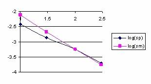
Figure 3. Logarithmical variation of the sum of positive (log(sp)) and negative(log(sm)) estimation errors depending on log(n) function for X/n = 1/2 fraction
Looking at the graphical representation from the figure 7 it can be observe that the variation of the errors sum was almost linear and inverse proportional with n. For the proportion X/n = 1/2 and generally for medium proportion the normal approximation is good and its quality increase with increasing of sample size (n). Moreover, to the surrounding of 1/2 the symmetry hypothesis of the confidence estimation induce by the normality approximation work perfectly.
Looking at the variation of the positive errors induced by the normal approximation for the proportion in form of X/n = 1/10 depending on n (see figure 4), it can be remarked that the abscissa of maximum point of deviation relative to binomial distribution are found at lower n in the vicinity of the extreme values. Thus, for n = 10, and X = 1 the error reach the maximum value of 0.108 at 0. The abscissa is moving towards X value with increasing of n (for n = 300, and X = 30 the error reach the maximum value of 0.0283 at 25).
For the variation of the negative errors induces by the normal approximation of the proportion of type X/n=1/10 depending on n, we can remark that the abscissa of maximum point of deviation depending on binomial distribution are found at lower n in the vicinity of the extreme values. Thus, for n = 10, and X = 3 the error reach the maximum value of 0.05 at 0. The abscissa is moving towards X value with increasing of n (for n = 300, and X = 30 the error reach the maximum value of 0.0260 at 34). More over, the approximation errors depending on X value is asymmetrical, and there was not any tendency for symmetry with increasing of n.
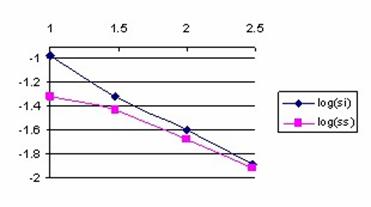
Figure 4. Logarithmic variation of the sum of values less than X (log(si)) and greater than X (log(ss)) depending on log(n) for X/n = 1/10 fraction
Because the sum of errors for values smaller than X were always greater than the sum of errors for the values greater than X, the confidence interval obtained base don normality approximation it will be displaced to the right (there were generate more approximation errors on the left side).
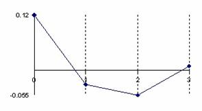
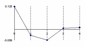
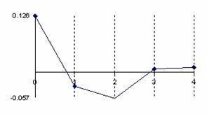
Figure 5. The error of binomial distribution approximate with a normal distribution with X/n = 1/n fraction express through Errc(n,1,Y) function at n = 10, n = 30, n = 100 and n = 300
The error had a maximum value of 10.8% for n = 10 and X = 1 into point 0, value which was greater twice than the accepted significance level α = 5% (!). A maximum value of 2.6% were obtained twice consecutively for n = 30, X = 3 into the 1 and 2 points and a maximum value of 2.5% into the point 4, that was half reported to the significance level α = 5% (!); which represent a sever deviation. For large n the sum of the approximation error there was a tendency to linearity inverse proportional with n.
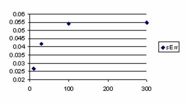
Figure 6. The variation of the error estimation sum for X/n = 1/n fraction
The graphical representations from the figure 5 and 6 reveal that for small proportions (X/n = 1/n) the sum of approximation errors were increasing with n. The sum of the approximation errors always exceeded the significance level (α = 5% (!)) for n > 50, which means that the real error threshold using normality hypothesis will exceeded 10%, the error being obtained in the favor of the greater values for the X.
Implementation of the Mathematical Calculation in MathCad
The experimental described in the previous section was possible after a MathCad implementation. The results obtained running the MathCad program were imports in Microsoft Excel were the graphical representations were creates.
In MathCad were implements the next functions:
· n combination taking to k: was necessary a logarithmical expression because we were working with large sample size and for n = 300 we could not used the classical formula C(n,k) = n!/((n-k)!k!)
 (7)
(7)
 (8)
(8)
 (9)
(9)
The calculation of Y/n apparition into a binomial distribution by n sample size and X/n proportion:
 (10)
(10)
The computing of the apparition of Y/n into a normal distribution sample by volume n, mean X/n and variance X(n-X)/n:
 (11)
(11)
The differences between the binomial and normal distribution:
 (12)
(12)
Initializations (needed for defining the series of values):
 (values which were consecutively changed with 10,1; 10,5; 30,1; 30,3; 30,15; 100,1; 100,10; 100,50; 300,1; 300,30; 300,150)

The computing of the series of corrected differences (graphically represented in figure 1, 2 and 5):
 (13)
(13)
The construction of the series of the positive sum of probabilities differences until to X (graphically represented in figure 3)
 (14)
(14)
The construction of the series of the positive sum of probabilities differences for the values less than X/n (graphically represented in figure 4)
 (15)
(15)
 - display the values of the sum for each pair of data
The calculation of the differences probabilities for every parameters:
 display the values of the sum for each pair of data (16)
Was also used a File Read/Write component (linked with dBNCY) in order to export the results into *.txt file from where the data were imported in Microsoft Excel where the graphical representation were drawing.
Generating a Binomial Sample using a PHP Program
In order to evaluate the confidence intervals for medical key parameters we decide to work with binomial samples and variables. In PHP was creates a module with functions that generates binomial distribution probabilities. Each by another, was implements functions for computing the binomial coefficient of n vs. k (bino0 function), the binomial probability for n, X, Y (bino1, bino2, and bino3 functions), drawing out a binomial sample of size n_es (bino4 function). Finally, array rearrangement of binomial sample values staring with position 0 and saving in the last element the value of rearrangement postponement are makes by bino5 function.
The used functions are:
function bino0($n,$k){ $rz = 1;
if($k<$n-$k) $k=$n-$k;
for ($j=1;$j<=$n-$k;$j++)
$rz *= ($k+$j)/$j;
return $rz; }
function bino1($n,$y,$x){ return pow($x/$n,$y)*pow(1-$x/$n,$n-$y)*bino0($n,$y); }
function bino2($n,$y,$x){
if(!$x) if($y) return 0; else return 1;
$nx=$n-$x; $ny=$n-$y;
if(!$nx) if($ny) return 0; else return 1;
$ret=0;
if($y){
$ret += log($x)*$y;
if($ny){
$ret += log($nx)*$ny;
if($ny>$y) $y=$ny;
for($k=$y+1;$k<=$n;$ret+=log($k++));
for($k=2;$k<=$n-$y;$ret-=log($k++)); }
} else $ret += log($nx)*$ny;
return exp($ret-log($n)*$n); }
function bino3($n,$y,$x){
if(!$x) if($y) return 0; else return 1;
$x/=$n; $nx=1-$x; $ny=$n-$y;
if(!$nx) if($ny) return 0; else return 1;
$ret=0;
if($y){
$ret += log($x)*$y;
if($ny){
$ret += log($nx)*$ny;
if($ny>$y) $y=$ny;
for($k=$y+1;$k<=$n;$ret+=log($k++));
for($k=2;$k<=$n-$y;$ret-=log($k++)); }
} else $ret += log($nx)*$ny;
return exp($ret); }
function bino4($n,$k,$n_es){
for($j=0;$j<=$n;$j++){
if($j>15) $c[$j]=bino1($n,$j,$k); else $c[$j]=bino3($n,$j,$k);
$c[$j]=round($c[$j]*$n_es);
if(!$c[$j])unset($c[$j]); }
return $c; }
function bino5($N,$k,$f_N){
$d=bino4($N,$k,$f_N);
$j=0;
foreach($d as $v) $r[$j++]=$v;
foreach($d as $i => $v) break;
$r[count($r)]=$i;
return $r; }
Computing the confidence intervals for a binomial variable is time consuming. In this perspective, an essential problem was optimizing the computing time. We studied comparative the time needed for generating the binomial probabilities using the bino1 function, the bino2 function, and the bino3 function. We developed a module which to collect and display the execution time. In the appreciation of the execution time, we used the internal clock of the computer.
The module that collects and displays the execution time is:
$af="N\tBino1\tBino2\tBino3\r\n";
for($n=$st;$n<$st+1;$n++){
$t1=microtime(TRUE);
for($x=0;$x<=$n;$x++) for($y=0;$y<=$n;$y++)
$b=bino1($n,$y,$x);
$t2=microtime(TRUE);
for($x=0;$x<=$n;$x++) for($y=0;$y<=$n;$y++)
$b=bino2($n,$y,$x);
$t3=microtime(TRUE);
for($x=0;$x<=$n;$x++) for($y=0;$y<=$n;$y++)
$b=bino3($n,$y,$x);
$t4=microtime(TRUE);
$af.=$n."\t";
$af.=sprintf("%5.3f",log((10000*($t2-$t1))))."\t";
$af.=sprintf("%5.3f",log((10000*($t3-$t2))))."\t";
$af.=sprintf("%5.3f",log((10000*($t4-$t3))))."\r\n";}
echo($af);
Table 1 contains the logarithmical values of the executions time for n: 3, 10, 30, 50, 100, 150, and 300 obtained by the bino1, bino2, and bino3 functions.
|
n
|
Bino1
|
Bino2
|
Bino3
|
|
3
|
1.92
|
1.573
|
1.406
|
|
10
|
3.975
|
4.021
|
3.956
|
|
30
|
6.441
|
6.763
|
6.74
|
|
50
|
7.731
|
8.149
|
8.137
|
|
100
|
9.576
|
10.108
|
10.101
|
|
150
|
10.706
|
11.28
|
11.278
|
|
300
|
12.691
|
13.314
|
13.314
|
Table 1. The execution time (seconds) express in logarithmical scale needed for generating binomial probabilities with implemented function
The differences between executions time express in logarithmical scale for the functions bino1and bino3 and respectively for the functions bino2 and bino3 were uses in order to obtain the graphical representations from the figure 7. Looking at the execution time ratio for the bino1 and bino3 function (the Bino2-Bino3 curve, figure 7) we can remark that optimizing parameter with X/n instead of X and (n-X)/n instead of (n-X) bring an increasing performance; this increased performance was cancel with increasing of n (the logarithmical difference was almost 0 for n >50).
Looking at the execution time ratio for the bino2 and bino3 functions (the Bino2-Bino3 curve, figure ) we can remark that with increasing of n the bino3 function obtained the best performance comparing with bino1 and bino2 (the differences between execution time express in logarithmical scale became less than 0 beginning with n ≈ 15). Based on above observations, was implements for the binomial probabilities estimation the bino4 function.
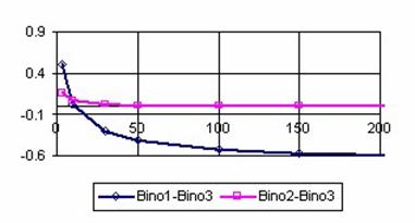
Figure 7. Binomial probabilities execution time for bino1, bino2, and bino3 functions
Medical Key Parameters on 2X2 Contingency Table
For the 2X2 contingency table data and based on the type of the medical studies we can compute some key parameters used for interpreting the studies results. Let us suppose that we have a contingency table as the one in the table 2.
|
|
| Result/Disease (Characteristic B)
|
|
|
| Positive
| Negative
| Total
|
|
Treatment / Risk factor / Diagnostic Test (Characteristic A)
|
Positive
|
a
|
b
|
a+b
|
|
Negative
|
c
|
d
|
c+d
|
|
Total
|
a+c
|
b+d
|
a+b+c+d
|
Table 2. Hypothetical 2X2 contingency table
In table 2, a denotes the real positive cases (those who have both characteristics), b the false positive cases (those who have just the characteristic A), c the false negative cases (those who have the characteristic B) and d the real negative cases (those who have neither characteristic).
We classified the medical key parameters based on the mathematical expressions (see table 3). This classification was very useful in confidence intervals assessment for each function, and for implementing the function in PHP.
The PHP functions for the mathematical expression described in the table 3 had the next expressions:
function ci1($X,$n){
return $X/$n; }
function ci2($X,$n){
if($X==$n) return (float)"INF";
return $X/($n-$X); }
function ci3($X,$n){
if(2*$X==$n) return (float)"INF";
return $X/(2*$X-$n); }
function ci4($X,$m,$Y,$n){
if(($X==$m)||($Y==0)) return (float)"INF";
return $X*($n-$Y)/$Y/($m-$X); }
function ci5($X,$m,$Y,$n){
return $Y/$n-$X/$m; }
function ci6($X,$m,$Y,$n){
return abs(ci5($X,$m,$Y,$n)); }
function ci7($X,$m,$Y,$n){
$val=ci6($X,$m,$Y,$n);
if(!$val) return (float)"INF";
return 1/$val; }
function ci8($X,$m,$Y,$n){
if($Y==0) return (float)"INF";
return ci1($X,$m)/ci1($Y,$n); }
function ci9($X,$m,$Y,$n){
if($Y==0) return (float)"INF";
return abs(1-ci1($X,$m)/ci1($Y,$n)); }
|
No
|
Mathematical expression and
PHP function
|
Name of the key parameter
|
Type of study
|
|
1
|
 , ci1 , ci1
| Individual Risk on Exposure Group and
NonExposure Group
|
Risk factor or prognostic factor studies [6], [7]
|
Experimental and Control Event Rates
Absolute Risk in Treatment and Control Group
|
Therapy studies [8], [9]
|
|
Sensitivity; Specificity; Positive and Negative Predictive Value; False Positive and Negative Rate; Probability of Disease, Positive and Negative Test Wrong; Overall Accuracy; Probability of a Negative and Positive Test
|
Diagnostic studies [10], [11], [12]
|
|
2
|
 , ci2 , ci2
|
Post and Pre Test Odds
|
Diagnostic studies 7, 9, 10]
|
|
3
|
 , ci3 , ci3
|
Post Test Probability
|
Diagnostic studies [9, 10]
|
|
4
|
 , ci4 , ci4
|
Odds Ratio
|
Risk Factor studies [6, 7]
|
|
5
|
 , ci5 , ci5
|
Excess risk
|
Risk Factor studies [5]
|
|
6
|
 , ci6 , ci6
|
Absolute Risk Reduction and Increase,
Benefit Increase
|
Therapy studies 7, 9]
|
|
7
|
 , ci7 , ci7
|
Number Needed to Treat and Harm
|
Therapy studies [7, 9]
|
|
8
|
 , ci8 , ci8
|
Relative Risk
|
Studies of Risk Factor [5, 6]
|
|
Positive and Negative Likelihood Ratio
|
Diagnostic studies [7, 9, 10]
|
|
9
|
 , ci9 , ci9
|
Relative Risk Reduction, Increase and
Benefit Increase
|
Therapy studies [7, 9]
|
Table 3. Mathematical expressions and PHP functions for medical key parameters
Estimating Confidence Intervals using a PHP program
In order to be able to check out if that the experimental numbers belong to confidence interval were implements in PHP two functions, one named out_ci_X for one-variable functions (depending on X) and the other, named out_ci_XY for two-variables functions (depending on X, Y). The functions had the expressions:
function out_ci_X(&$cif,$XX,$X,$n,$z,$a,$f,$g){
$ci_v=ci($cif,$g,$X,$n,$z,$a);
if(!is_finite($ci_v[1])) return 0;
if(!is_finite($ci_v[0])) return 0;
$ci_v=ci($cif,$g,$XX,$n,$z,$a);
if(!is_finite($ci_v[1])) return 0;
if(!is_finite($ci_v[0])) return 0;
$fx=$f($X,$n);
if(!is_finite($fx)) return 0;
return (($fx<$ci_v[0])||($fx>$ci_v[1]));}
function out_ci_XY(&$cif,$XX,$X,$YY,$Y,$m,$n,$z,$a,$f){
$ci_v=$cif($XX,$m,$YY,$n,$z,$a);
if(!is_finite($ci_v[0])) return 0;
if(!is_finite($ci_v[1])) return 0;
$fxy=$f($X,$m,$Y,$n);
if(!is_finite($fxy)) return 0;
return (($fxy<$ci_v[0])||($fxy>$ci_v[1]));}
The function est_ci_er compute the confidence interval boundaries, the experimental errors, the mean, and the standard deviation for the expression with one variable (X); the est_ci2_er was the function for the two-variable expressions (X, Y):
function est_ci_er($z,$a,$c_i,$g,$f,$ce){
if($ce=="ci") est_X(z,a,$c_i,$f,$g);
if($ce=="er") est_N(z,a,$c_i,$f,$g,1);
if($ce=="me") est_N(z,a,$c_i,$f,$g,2);
if($ce=="va") est_N(z,a,$c_i,$f,$g,3);
if($ce=="mv") est_N(z,a,$c_i,$f,$g,6);}
function est_ci2_er($z,$a,$c_i,$f,$ce){
if($ce=="ci") est_X2(z,a,$c_i,$f);
if($ce=="er") est_N2(z,a,$c_i,$f);
if($ce=="me") est_MN(z,a,$c_i,$f,2);
if($ce=="va") est_MN(z,a,$c_i,$f,3);
if($ce=="mv") est_MN(z,a,$c_i,$f,6);}
The est_X compute all the confidence intervals for the one-variable functions (depending on X) while est_X2 compute the confidence intervals for two-variable functions (depending on X, Y):
function est_X($z,$a,$c_i,$f,$g){
echo("N\tX\tf(X)");
for($i=0;$i<count($c_i);$i++){
echo("\t".$c_i[$i]."L");
echo("\t".$c_i[$i]."U"); }
for($n=N_min;$n<N_max;$n++){
for($X=0;$X<=$n;$X++){
for($i=0;$i<count($c_i);$i++)
$ci[$i] = ci($c_i[$i],$g,$X,$n,$z,$a);
$fX = $f($X,$n);
echo("\r\n".$n."\t".$X."\t".trim(sprintf("%6.3f",$fX)));
for($k=0;$k<count($c_i);$k++){
echo("\t".trim(sprintf("%6.3f",$ci[$k][0])));
echo("\t".trim(sprintf("%6.3f",$ci[$k][1]))); } }}}
function est_X2($z,$a,$c_i,$f){
echo("X\tY\tf(X,Y)");
for($i=0;$i<count($c_i);$i++){
echo("\t".$c_i[$i]."L");
echo("\t".$c_i[$i]."U"); }
for($n=N_min;$n<N_max;$n++){
$m = $n;
for($X=0;$X<=$m;$X++){
for($Y=0;$Y<=$n;$Y++){
for($i=0;$i<count($c_i);$i++){
$g = $c_i[$i];
$ci[$i] = $g($X,$m,$Y,$n,$z,$a); }
$fXY = $f($X,$m,$Y,$n);
echo("\r\n".$X."\t".$Y."\t".trim(sprintf("%6.3f",$fXY)));
for($k=0;$k<count($c_i);$k++){
echo("\t".trim(sprintf("%6.3f",$ci[$k][0])));
echo("\t".trim(sprintf("%6.3f",$ci[$k][1]))); } } } }}
The est_N function computed the estimation errors or means or/and standard deviations of the mean for the one-variable functions (depending on X); the est_N2 function computed the estimation errors for two-variable functions (depending on X, Y):
function est_N($z,$a,&$c_i,$cif,$g,$ce){
if($ce==1)echo("N\tX\tf(x)");else echo("N");
for($i=0;$i<count($c_i);$i++)
echo("\t".$c_i[$i]);
for($n=N_min;$n<N_max;$n++){
for($X=1;$X<p*$n;$X++){
$d=bino4($n,$X,10000);
if($ce==1) echo("\r\n".$n."\t".$X."\t".trim(sprintf("%6.3f",$cif($X,$n))));
for($i=0;$i<count($c_i);$i++){//pt fiecare ci
$ttt[$X][$i]=0;//esecuri
$conv=0;
foreach ($d as $XX => $nXX){//pt fiecare valoare posibila de esantion
if(out_ci_X($c_i[$i],$XX,$X,$n,$z,$a,$cif,$g)) $ttt[$X][$i] += $nXX;
$conv += $nXX; }
$ttt[$X][$i] *= 100/$conv;
if($ce==1)echo("\t".trim(sprintf("%3.3f",$ttt[$X][$i]))); } }
if ($ce > 1) est_MV($ttt,count($c_i),$n,p,0,$ce,$a); }}
function est_N2($z,$a,&$c_i,$f){
echo("X\tY\tf(X,Y)");
for($i=0;$i<count($c_i);$i++)
echo("\t".$c_i[$i]);
for($n=N_min;$n<N_max;$n++){
$m = $n;
for($X=1;$X<p*$m;$X++){
$dX=bino4($m,$X,1000);
for($Y=1;$Y<p*$n;$Y++){
$dY=bino4($n,$Y,1000);
echo("\r\n".$X."\t".$Y."\t".trim(sprintf("%3.3f",$f($X,$m,$Y,$n))));
for($i=0;$i<count($c_i);$i++){
$ttt[$X][$Y][$i]=0;//esecuri
$conv=0;
foreach ($dX as $XX => $nXX){
foreach ($dY as $YY => $nYY){
if(out_ci_XY($c_i[$i],$XX,$X,$YY,$Y,$m,$n,$z,$a,$f))
$ttt[$X][$Y][$i] += $nXX*$nYY;
$conv += $nXX*$nYY; } }
echo("\t".trim(sprintf("%3.3f",100*$ttt[$X][$Y][$i]/$conv))); } } } }}
The est_MN function computed the means and/or the standard deviations of the mean for the two-variable functions (depending on X, Y):
function est_MN($z,$a,&$c_i,$f,$ce){
echo("M\tN");
for($i=0;$i<count($c_i);$i++)
echo("\t".$c_i[$i]);
for($m=N_min;$m<N_max;$m++){
for($n=N_min;$n<N_max;$n++){
for($i=0;$i<count($c_i);$i++){
if($ce % 2 == 0) $md[$i] = 0;
if($ce % 3 == 0) $va[$i] = 0; }
for($X=1;$X<p*$m;$X++){
$dX=bino4($m,$X,10000);
for($Y=1;$Y<p*$n;$Y++){
$dY=bino4($n,$Y,10000);
for($i=0;$i<count($c_i);$i++){
$ttt[$X][$Y][$i]=0;//esecuri
$conv=0;
foreach ($dX as $XX => $nXX){
foreach ($dY as $YY => $nYY){
if(out_ci_XY($c_i[$i],$XX,$X,$YY,$Y,$m,$n,$z,$a,$f))
$ttt[$X][$Y][$i] += $nXX*$nYY;
$conv += $nXX*$nYY; } }
if($ce % 2 == 0) $md[$i] += 100*$ttt[$X][$Y][$i]/$conv;
if($ce % 3 == 0) $va[$i] += pow(100*$ttt[$X][$Y][$i]/$conv-5,2); } } }
echo("\r\n".$m."\t".$n);
for($i=0;$i<count($c_i);$i++){
if($ce % 2 == 0)
echo("\t".trim(sprintf("%3.3f",$md[$i]/($m-1)/($n-1))));
if($ce % 3 == 0)
echo("\t".trim(sprintf("%3.3f",sqrt($va[$i]/(($m-1)*($n-1)-1))))); } } }}
The est_MV function computed the estimation errors means and/or standard deviations:
function est_MV(&$ttt,$n_c_i,$n,$p,$v,$ce,$a){
for($i=0;$i<$n_c_i;$i++){
$md[$i]=$v; if($v)continue;
if($p==0.5){
for($X=1;$X<$p*$n;$X++) $md[$i]+=2*$ttt[$X][$i];
if(is_int($p*$n)) $md[$i]+=$ttt[$p*$n][$i];
$md[$i]/=($n-1);
} else {
for($X=1;$X<$p*$n;$X++) $md[$i]+=$ttt[$X][$i];
$md[$i]/=($n-1); } }
if($ce % 3 == 0)
for($i=0;$i<$n_c_i;$i++){
$ds[$i]=0;
if($p==0.5){
for($X=1;$X<$p*$n;$X++){
$ds[$i]+=2*pow($ttt[$X][$i]-$md[$i],2); }
if(is_int($p*$n)) $ds[$i]+=pow($ttt[$X][$i]-100*$a,2);//$md[$i],2);
$ds[$i]/=($n-2);//s
$ds[$i]=pow($ds[$i],0.5);
} else {
for($X=1;$X<$p*$n;$X++){
$ds[$i]+=pow($ttt[$X][$i]-100*$a,2);//$md[$i],2); }
$ds[$i]/=($n-2);//s
$ds[$i]=pow($ds[$i],0.5); } }
if($ce % 2 == 0){
echo("\r\n".$n);
for($i=0;$i<$n_c_i;$i++)
echo("\t".trim(sprintf("%3.3f",$md[$i]))); }
if($ce % 3 == 0){
echo("\r\n".$n);
for($i=0;$i<$n_c_i;$i++)
echo("\t".trim(sprintf("%3.3f",$ds[$i]))); }}
The est_R2 function compute and display, for a 100 random sample size and binomial variables values the experimental errors using the imposed (theoretical) value of significance level for all confidence interval calculation methods given also as parameter:
function est_R2($z,$a,&$c_i,$f){
echo("p\tM\tN\tX\tY\tf(X,Y)");
for($i=0;$i<count($c_i);$i++)
echo("\t".$c_i[$i]);
for($k=0;$k<100;$k++){
$n = rand(4,1000);
$m = rand(4,1000);
$X = rand(1,$m-1);
$Y = rand(1,$n-1);
$dX=bino4($m,$X,10000);
$dY=bino4($n,$Y,10000);
echo("\r\n".$k."\t".$m."\t".$n."\t".$X."\t".$Y."\t".trim(sprintf("%3.3f",$f($X,$m,$Y,$n))));
for($i=0;$i<count($c_i);$i++){//pt fiecare ci
$ttt[$X][$Y][$i]=0;//esecuri
$conv=0;
foreach ($dX as $XX => $nXX){
foreach ($dY as $YY => $nYY){
if(out_ci_XY($c_i[$i],$XX,$X,$YY,$Y,$m,$n,$z,$a,$f))
$ttt[$X][$Y][$i] += $nXX*$nYY;
$conv += $nXX*$nYY;
}
}
echo("\t".trim(sprintf("%3.3f",100*$ttt[$X][$Y][$i]/$conv)));
}
}
}
The est_C2 function compute and display for a fixed value of proportion X/n (usually the central point X/n = 1/2) the errors for a series of sample size (from N_min to N_max):
function est_C2($z,$a,&$c_i,$f){
echo("X\tY\tf(X,Y)");
for($i=0;$i<count($c_i);$i++)
echo("\t".$c_i[$i]);
for($n=N_min;$n<N_max;$n+=4){
$m = $n;
//$X = (int)(3*$m/4); $Y = (int)($n/4);
$X = (int)($m/2); $Y = (int)($n/2);
$dX=bino4($m,$X,10000);
//$dY=bino4($n,$Y,10000);
$dY=$dX;
echo("\r\n".$X."\t".$Y."\t".trim(sprintf("%3.3f",$f($X,$m,$Y,$n))));
for($i=0;$i<count($c_i);$i++){
$ttt[$X][$Y][$i]=0;//esecuri
$conv=0;
foreach ($dX as $XX => $nXX){
foreach ($dY as $YY => $nYY){
if(out_ci_XY($c_i[$i],$XX,$X,$YY,$Y,$m,$n,$z,$a,$f))
$ttt[$X][$Y][$i] += $nXX*$nYY;
$conv += $nXX*$nYY;
}
}
echo("\t".trim(sprintf("%3.3f",100*$ttt[$X][$Y][$i]/$conv)));
}
}
}
The ci function used in est_N, est_N2, est_X, and est_X2 functions compute the confidence interval for specified function with specified parameter and it was uses for the nine functions described in table 3. Corresponding to the functions described in table 3, were defines:
the I function for the expression X/n;
the R function was used for the expression X/(n-X);
the RD function was used for the expression X/(2X-n);
the R2 function for the expression X(n-Y)/Y/(m-X);
the D function for the expression Y/n-X/n;
the AD function for the expression |Y/n-X/n|;
the IAD function for the expression 1/|Y/n-X/n|;
the RP function for the expression Xn/Y/m;
the ARP function for the expression |1- Xn/Y/m|.
For the one-variable expressions (f(X)) the confidence intervals was compute using the next expressions:
For ci1 function:
o Mathematical expression:  (17)
(17)
where CIL(X) and CIU(X) were the lower limit and respectively the upper limit of the confidence interval;
o PHP function:
function I($f,$X,$n,$z,$a){
return $f($X,$n,$z,$a);}
For ci2 function:
o Mathematical expression:  (18)
(18)
o PHP function:
function R($f,$X,$n,$z,$a){
$L = $f($X,$n,$z,$a);
if ($L[1])
if ($L[1]-1) $Xs = 1/(1/$L[1]-1); else $Xs = (float) "INF";
else $Xs = 0;
if ($L[0]-1)
if ($L[0]) $Xi = 1/(1/$L[0]-1); else $Xi = 0;
else $Xi = 0;
return array ( $Xi , $Xs );}
For ci3 function; the expression for confidence interval is based on confidence intervals expression used for ci1:
o Mathematical expression:  (19)
(19)
o PHP function:
function RD($f,$X,$n,$z,$a){
if($X==$n-$X) return array( -(float)"INF" , (float)"INF" );
$q=$f($X,$n,$z,$a);
if($X==$n) return array ( 1/$q[1] , 1/$q[0] );
if($q[0]==0) $tXs = 0; else $tXs = 1/(2-1/$q[0]);
if($q[1]==0.5)
$tXi=-(float)"INF";
else if(!$q[1])
$tXi=0;
else
$tXi = 1/(2-1/$q[1]);
if($X){
$tX= 1/(2-$n/$X);
if(($tXi>$tX)||($tXs<$tX)) {
$tnX=1/(2-$n/($n-$X));
if(abs($tnX)<abs($tX))$tX=$tnX;
$tXi = $tX * exp(exp(abs($tX)));
$tXs = -$tX * exp(exp(abs($tX))); } }
return array( $tXi , $tXs );}
The formulas for computing the confidence intervals for two-variable functions (depending on X, Y) can be express base on the formulas for confidence intervals of one-variable functions (depending on X):
For ci4 function:
o Mathematical expression:  (20)
(20)
o PHP function:
function R2($f,$X,$m,$Y,$n,$z,$am,$an){
$ciX = R($f,$X,$m,$z,$am);
$cinY = R($f,$n-$Y,$n,$z,$an);
return array ( $ciX[0]*$cinY[0] , $ciX[1]*$cinY[1] );}
For ci5 function:
o Mathematical expression:  (21)
(21)
o PHP function:
function D($f,$X,$m,$Y,$n,$z,$am,$an){
$ciX = $f($X,$m,$z,$am);
$ciY = $f($Y,$n,$z,$an);
return array ( $ciY[0]-$ciX[1] , $ciY[1]-$ciX[0] );}
For ci6 function:
o Mathematical expression:
 (22)
(22)
o PHP function:
function AD($ci){
if($ci[0]*$ci[1]<=0){
$max =abs($ci[0]);
if($max<abs($ci[1])) $max = abs($ci[1]);
return array ( 0 , $max );
}else{
if($ci[0]<0) {
$ci[0] = abs($ci[0]);
$ci[1] = abs($ci[1]); }
if($ci[0]<$ci[1]) return array( $ci[0] , $ci[1] );
else return array( $ci[1] , $ci[0] ); }}
For ci7 function:
o Mathematical expression:  (23)
(23)
o PHP function:
function IAD($CI){
if($CI[0]) $Xs = 1/$CI[0]; else $Xs = (float)"INF";
if($CI[0]) $Xi = 1/$CI[1]; else $Xi = (float)"INF";
return array( $Xi , $Xs );}
For ci8 function:
o Mathematical expression:  (24)
(24)
o PHP function:
function RP($f,$X,$m,$Y,$n,$z,$am,$an){
$ciX = $f($X,$m,$z,$am);
$ciY = $f($Y,$n,$z,$an);
$XYi = $ciX[0]/$ciY[1];
if($ciY[0]) $XYs = $ciX[1]/$ciY[0]; else $XYs = (float)"INF";
return array ( abs($XYi), $XYs );}
For ci9 function:
o Mathematical expression:

o PHP function:
function ARP($f,$X,$m,$Y,$n,$z,$a){
$ci = $f($X,$m,$Y,$n,$z,$a);
if(!is_finite($ci[1])) return array ( abs(1-$ci[0]) , (float)"INF" );
$t1 = 1-$ci[0];
$t2 = 1-$ci[1];
if($t1*$t2<=0){
$Xi = 0;
if(abs($t2)>abs($t1))
return array( 0 , abs($t2) );
else
return array( 0 , abs($t1) );
}else{
if(abs($t2)>abs($t1))
return array ( abs($t1) , abs($t2) );
else
return array ( abs($t2) , abs($t1) ); }}
Were defined the normal distribution percentile (z), the error of the first kind or the significance level (a), the value for the maximum proportion for which the confidence intervals was estimated (p), the sample sizes start value (N_min) and the sample sizes stop value (N_max):
define("z",1.96);
define("a",0.05);
define("p",1);
define("N_min",10);
define("N_max",11);
A specific PHP program calls all these functions for a given n and display the estimation errors or confidence intervals limits at a specified significance level (α =5%) using est_ci_er or est_ci2_er functions. For example, in order to compute the confidence interval for a proportion (ci1 function) was call the est_ci_er function with the next parameters:
est_ci_er(z,a,$c_i,"I","ci1","ci");
where $c_i was a matrix that memorize the name of the methods used in confidence intervals estimation and I was the name of the function defined above for the expression X/n.
In the next articles, we will debate the confidence intervals methods for each function described in table 1 and their variability with sample size.
The standard deviation of the experimental error was computes using the next formula:
 (26)
(26)
where StdDev(X) is standard deviation, Xi is the experimental errors for a given i (0 ≤ i ≤ n), M(X) is the arithmetic mean of the experimental errors and n is the sample size.
If we have a sample of n-1 elements (withdrawing the limits 0 and n from the 0..n array) with a known (or expected) mean ExpM(X), the deviation around α = 5% (imposed significance level) is giving by:
 (27)
(27)
The (27) formula was used as a quantitative measure of deviation of errors relative to imposed error value (equal with 100α) when ExpM(X) = 100α.
Two-dimensional Functions
We used the uni-dimensional (X, m) confidence intervals functions to compute the confidence intervals for bi-dimensional functions (X, m, Y, n) but were necessary to perform a probability correction. We consider that the confidence intervals boundaries of bi-dimensional functions were gives by the product of the limits from the uni-dimensional cases with a correction of the significance level based on error convolution product.
Experimentally was infers that the best expression for the significance level for bi-dimensional function was:
 or, with correction by m,
  (26)
(26)
where a was the uni-dimensional significance level and aU şi aU(m) were imposed significance level for uni-dimensional variable (X) with a volume m. Analogue can be obtained the expression for the uni-dimensional variable (Y) with a volume n, aU(n).
Random Sampling
We consider 100 random values for n and respectively for m in the 4..1000 domain and X, respectively Y in domain 1..m-1, respectively 1..n-1. The error estimation of the confidence interval was performs for these samples and the results were graphically represented using MathCad program. Thus, we implement a module in MathCad that allowed us to perform these representations using:
The frequencies of experimental errors;
Dispersion relative to the imposed error value (α = 5%);
The mean and standard deviation of the experimental errors;
The theoretical errors distribution graphic based on Gauss distribution of means equal with five (significance level α = 5%) and standard deviation equal with a standard deviation of a volume sample size equal width 10 (double of α).
The corresponding equations are:
 (27)
(27)
 (28)
(28)
 (29)
(29)
 (30)
(30)
 (31)
(31)
 (32)
(32)
 (33)
(33)
 (34)
(34)
 (35)
(35)
 (36)
(36)
 (37)
(37)
 (38)
(38)
 (39)
(39)
 (40)
(40)
 (41)
(41)
 (42)
(42)
Graphical Representations
We developed a graphical module in PHP for graphical error map representations for bi-dimensional functions (X, m). The module used the confidence intervals computed by the program described above and performs (m, X, Z) graphical representations, where Z can be the value of the confidence intervals or the estimation errors (percentages) and perform a triangular graphical representation for Z (X on the horizontal axis; m on the vertical axis, descending order) using a color gradient. The module lines were:
<?
define("pct",3);
define("fmin",0);
define("fmax",10);
define("ncol",21);
define("tip",1);
$file="BayesF";
g_d($file,$v);
i_p($file,$v);
function i_p(&$file,&$v){
$in=pct*($v[count($v)-1][0]+1);
$image = @imagecreate($in, $in);
$alb = imagecolorallocate($image,255,255,255);
$negru = imagecolorallocate($image,0,0,0);
$t_l = $in-imagefontwidth(2)*strlen($file)-10;
imagestring($image, 2, $t_l,10, $file, $negru);
$cl = s_c_t($image,tip);
for($k=0;$k<count($v);$k++)
for($i=0;$i<pct;$i++){
for($j=0;$j<pct;$j++){
imagesetpixel($image,pct*$v[$k][1]+$i,pct*$v[$k][0]+$j,$cl[c($v[$k][2])]); } }
imagepng($image);
//imagegif($image);
//imageinterlace($image,1);imagejpeg($image); }
function c($z){
if($z<=fmin) return 1;
if($z>=fmax) return ncol-1;
$cu = ($z-fmin)*(ncol-3)/(fmax-fmin);
$cu = (int)$cu;
return $cu + 1;}
function g_d($file,&$v){
$data=file_get_contents($file.".txt");
$r=explode("\r\n",$data);
for($i=0;$i<count($r);$i++) $v[$i]=explode("\t",$r[$i]);}
function s_c_t(&$image,$tip){
if($tip==0){//negru-alb
for ($i=0;$i<ncol;$i++){
$cb=round($i * 255/(ncol-1));
$tc[$i]=array( $cb , $cb , $cb ); } }
if($tip==1){//rosu-albastru
$tc[0] = array( 255 , 0 , 0 );
$yl = (ncol-1)/2; $yl = (int) $yl;
if($yl>1)
for($i=1;$i<$yl;$i++){
$cb = round($i * 255/$yl);
$tc[$i] = array( 255 , $cb , 0 ); }
$tc[$yl] = array( 255 , 255 , 0 );
if($yl>1)
for($i=1;$i<$yl;$i++){
$cb = round($i * 255/$yl);
$tc[$yl+$i] = array( 255-$cb , 255-$cb , $cb ); }
$tc[ncol-1] = array( 0 , 0 , 255 ); }
if($tip==2){//rosu-verde
$tc[0] = array( 255 , 0 , 0 );
$yl = (ncol-1)/2; $yl = (int) $yl;
if($yl>1)
for($i=1;$i<$yl;$i++){
$cb = round($i * 255/$yl);
$tc[$i] = array( 255 , $cb , 0 ); }
$tc[$yl] = array( 255 , 255 , 0 );
if($yl>1)
for($i=1;$i<$yl;$i++){
$cb = round($i * 255/$yl);
$tc[$yl+$i] = array( 255-$cb , 255 , 0 ); }
$tc[ncol-1] = array( 0 , 255 , 0 ); }
for ($k=0;$k<ncol;$k++)
$cl[$k]=imagecolorallocate($image,$tc[$k][0],$tc[$k][1],$tc[$k][2]);
return $cl;}
?>
The module describe above used the pct (= 3) constant in order to represent a 3×3 pixeli square for each m, X, color(Z). The constant fmin was used to represent the values between the lower limit color (red color in our representations) and the middle limit color (yellow in our representations); the fmax constant was used to represent the maximum values which color were between upper limit color (blue) and middle limit color (yellow). All the values which not belong to the fmin , fmax] domain were represented with the lower limit color (if Z < fmin) or upper limit color (if Z > fmax). The number of shade (including the based color represented by red, yellow and blue) were defined by n_col constant (was chosen 21). The tip constant (was choose 1) define the couplet of the limit color and the corresponding shade using 3 couplet sets defined as follows: (White, Gray, Black), (Red, Yellow, Blue), and (Red, Yellow, Green).
Discussions
The approximation to normality of a binomial distribution had major disadvantages more obvious to the extremities of the proportion (X/n → 0 and X/n → 1).
Comparing different probability distribution functions revealed significant differences performances with increasing of n. The best performance methods were the functions that apply first direct and then inverse the logarithmical expression of the binomial probability function. Defining the key parameters as mathematical functions depending on random variable and sample size restrict the number of inquisition of theirs confidence intervals (from 34 medical key parameters to 9 distinct mathematical expression) (see table 3).
Working with PHP programming language offer a maximum flexibility in:
1defining and using the medical key parameters;
2defining and generating the binomial samples;
3performing the experimental of computing the confidence intervals limits;
4computing the experimental errors for each defined confidence interval methods.
For the medical key parameters, the confidence intervals expression of the parameters which depend on two random variable (X, Y) and two sample sizes (m, n) can be express based on the confidence intervals expressions for a proportion with changing the imposed value of probability.
MathCad program proved very useful in the situation were was necessary to perform complex integrals and to represent graphically the results, how was the case of the integrals based on expressions of the Gaussian function (f(x)=a∙exp((x-b)2/c2) [13]).
The tree dimensional graphical representations of the functions with two parameters (most of the medical key parameters), where the expression of the confidence intervals function of f(X,m), need a triangular grid (0 ≤ X ≤ n, were n vary on a specified domain - 4..103). There are a few software which to allow to represent correctly these kind of triangular plots, most of the software used some interpolation functions and the graphical representation are square plots (0 ≤ X ≤ 103; 4 ≤ n ≤ 103) instead of triangular plots (0 ≤ X ≤ n; 4 ≤ n ≤ 103). Thus was necessary to used PHP in order to create correct error maps.
All the aspects presented in this paper uses in the confidence intervals estimations for the key parameters used as measure the effect size for different healthcare intervention express as different medical key parameters (see further papers).
References
[1]. Huw D., What are confidence intervals?, What is
, Hayward Group Publication, 2003, 3, p. 1-9, available at: http://www.evidence-based-medicine.co.uk/ebmfiles/WhatareConfInter.pdf
[2]. Easton V.J., McColl H.J., Confidence intervals from Statistics Glossary v1.1, available at: http://www.cas.lancs.ac.uk/glossary_v1.1/confint.html
[3]. Bland M., Probability, chapter from An Introduction to Medical Statistics, Oxford Medical Publications, Oxford - New York - Tokyo, 1996, p. 86-99.
[4]. Abraham Moivre, The Doctrine of Chance: or The Method of Calculating the Probability of Events in Play, W. Pearforn, Second Edition, 1738.
[5]. K. Pawlikowski D.C., McNickle G.E., Coverage of Confidence Intervals in Sequential Steady-State Simulation, Simulation Practice and Theory, 1998, 6, p. 255-267.
[6]. Drugan T., Bolboacă S., Colosi H., Achimaş Cadariu A., Ţigan Ş., Dignifying of prognostic and Risc Factors Chapter in Statistical Inference of Medical Data, ALMA MATER Cluj-Napoca, 2003, p. 66-71 (in Romanian).
[7]. Sackett D.L., Straus S., Richardson W.S., Rosenberg W., Haynes R.B., Diagnosis and screening Chapter In Evidence-based medicine. How to practice and teach EBM, Second Ed., Edinburgh, Churchill Livingstone, 2000, p. 67-93.
[8]. Achimaş Cadariu A., Evidence Based Gastroenterology Chapter from Grigorescu M., Treaty of Gastroenterology, Medical National Publishing House, Bucharest, 2001, p. 629-659 (in Romanian).
[9]. Sackett D., Straus E.S., Richardson W.S., Rosenberg W., Haynes R.B., Therapy Chapter In: Evidence-based Medicine: How to Practice and Teach EBM, 2nd Ed., Edinburgh, Churchill Livingstone, 2000, p. 105-154.
[10]. Achimaş Cadariu A., Diagnostic Procedure Assessment Chapter from Achimaş Cadariu A. Scientific Medical Research Methodology, Medical University Iuliu Haţieganu Publishing House, Cluj-Napoca, 1999, p. 29-38 (in Romanian).
[11]. Hamm R. M., Clinical Decision Making Spreadesheet Calculator, University of Oklahoma Health Sciences Center, available at:www.emory.edu/WHSC/MED/EMAC/curriculum/diagnosis/oklahomaLRs.xls
[12]. Epidemiology&Lab Statistics from Study Counts, EpiMax Table Calculator, Princeton, New Jersey, USA, available at: http://www.healthstrategy.com/epiperl/epiperl.htm
[13]. TheFreeDictionary.com, Gaussian function, available at: http://encyclopedia.thefreedictionary.com/Gaussian function
Issue 03, p. 075-110
Binomial Distribution Sample Confidence Intervals Estimation 2. Proportion-like Medical Key Parameters
Sorana BOLBOACĂ*, Andrei ACHIMAŞ CADARIU
Iuliu Haţieganu University of Medicine and Pharmacy, Cluj-Napoca, Romania
* corresponding author, sbolboaca@umfcluj.ro
Abstract
The accuracy of confidence interval expressing is one of most important problems in medical statistics. In the paper was considers for accuracy analysis from literature, a number of confidence interval formulas for binomial proportions from the most used ones.
For each method, based on theirs formulas, were implements in PHP an algorithm of computing.
The performance of each method for different sample sizes and different values of binomial variable was compares using a set of criteria: the average of experimental errors, the standard deviation of errors, and the deviation relative to imposed significance level. A new method, named Binomial, based on Bayes and Jeffreys methods, was defines, implements, and tested.
The results show that there is no method from considered ones, which to have a constant behavior in terms of average of the experimental errors, the standard deviation of errors, or the deviation relative to imposed significance level for every sample sizes, binomial variables, or proportions of them. More, this unfortunately behavior remains also for large and small subsets of natural numbers set. The Binomial method obtained systematically lowest deviations relative to imposed significance level (α = 5%) starting with a certain sample size.
Keywords
Confidence Intervals; Binomial Proportion; Proportion-like Medical Parameters
Introduction
In the medical studies, many parameters of interest are compute in order to assess the effect size of healthcare interventions based on 2X2 contingency table and categorical variables. If we look for example at diagnostic studies, we have the next parameters that can be express as a proportion: sensitivity, specificity, positive predictive value, negative predictive value, false negative rate, false positive rate, probability of disease, probability of positive test wrong, probability of negative test wrong, overall accuracy, probability of a negative test, probability of a positive test [1], [2], [3]. For the therapy studies experimental event rate, control event rate, absolute risk in treatment group, and absolute risk on control group are the proportion-like parameter [4], [5] which can be compute based on 2X2 contingency table. If we look at the risk factor studies, the individual risk on exposure group and individual risk on nonexposure group are the parameters of interest because they are also proportions [6]. Whatever the measure used, some assessment must be made of the trustworthiness or robustness of the findings, even if we talk about a p-value or confidence intervals. The confidences intervals are preferred in presenting of medical results because are relative close to the data, being on the same scale of measurements, while the p-values is a probabilistic abstraction [7]. Rothmans sustained that confidence intervals convey information about magnitude and precision of effect simultaneously, keeping these aspects of measurement closely linked [8]. The confidence intervals estimation for a binomial proportion is a subject debate in many scientific articles even if we talk about the standard methods or about non asymptotic methods [9], [10], [11], [12]. It is also known that the coverage probabilities of the standard interval can be erratically poor even if p is not near the boundaries 10, [13], [14], [15]. Some authors recommend that for the small sample size n (40 or less) to use the Wilson or the Jeffreys confidence intervals method and for the large sample size n (> 40) the Agresti-Coull confidence intervals method [10].
The aim of this research was to assess the performance for a binomial distribution samples of literature reported confidence intervals formulas using a set of criterions and to define, implement, and test the performance of a new original method, called Binomial.
Materials and Methods
In literature, we found some studies that present the confidence intervals estimation for a proportion based on normal probability distribution or on binomial probability distribution, or an binomial distribution and its approximation to normality [16].
In this study, we compared some confidence intervals expressions, which used the hypothesis of normal probability distribution, and some confidence intervals formula, which used the hypothesis of binomial probability distribution. It is necessary to remark that the assessment of the confidence intervals, which used the hypothesis of binomial distribution, is time-consuming comparing with the methods, which used the hypothesis of a normal distribution.
In order to assess, both confidence intervals estimation aspects, quantitative and qualitative, and the performance of a confidence interval comparative with other methods we developed a module in PHP. The module was able to compute and evaluate the confidence intervals for a given X and a given n, build up a binomial distribution sample (XX) based on given X and compute the experimental errors of X values into its confidence intervals of xx from XX for each specified methods. We choose in our experiments a significance level equal with α = 5% (α = 0.05; noted a in our program) and the corresponding normal distribution percentile z1-α/2 = 1.96 (noted z in the program) for the confidence intervals which used normal distribution probability. The value of sample size (n) was chosen in the conformity with the real number from the medical studies; in our experiments, we used 4 ≤ n ≤ 1000. The estimation of the errors were performed for the value of X variable which respect the rule 0 < X < n. The confidence intervals used in this study, with their references, are in table 1. The confidence intervals presented in table 1 were not the all methods used in confidence intervals estimation for a proportion but they are the methods most frequently reported in literature.
Note that the performance of confidence interval calculation is dependent on method formula and eventually sample size and it must be independent on binomial variable value. Repetition of the experiment will and must produce same values of percentage errors for same binomial variable value, sample size, and method of calculation.
|
No
|
Methods
|
Lower and upper confidence limits
|
|
1
|
Wald
[1]
|
 ; c = 0 (standard); c = 0.5 (continuity correction) ; c = 0 (standard); c = 0.5 (continuity correction)
|
|
2
|
Wilson
[10]
|
 ; ;
Continuity correction: 

|
|
3
|
ArcSine
[17]
|
 or 0 (X = 0) or 1 (X = n) (ArcS) or 0 (X = 0) or 1 (X = n) (ArcS)
Continuity correction methods:
 (ArcSC1) (ArcSC1)
 (ArcSC2) (ArcSC2)
 (ArcSC3) (ArcSC3)
|
|
4
|
Agresti-Coull
[10]
|

|
|
5
|
Logit
[10]
|
 for 0 < X < n; Continuity correction: for 0 < X < n; Continuity correction:

|
|
6
| Binomial distribution methods
[10,17]
Clopper-Pearson
Jeffreys
Bayesian, BayesianF
Blyth-Still-Casella
[18], [19]
|
for 0 < X < n we define the function:
BinI(c1,c2,a) = 
BinS(c1,c2,a) = 
Clopper-Pearson: BinI(0,1,α/2), BinS(0,1,α/2) or 0 (X=0), 1(X=n)
Jeffreys: BinI(0.5,0.5,α/2), BinS(0.5,0.5,α/2)
BayesianF: BinI(1,1,α/2), BinS(1,1,α/2) or 0 (X=0), 1(X=n)
Bayesian: BinI(1,1,α/2) or 0 (X=0) , α1/(n+1) (X=n),
BinS(1,1,α/2) or 1- α1/(n+1) (X=0) , 1 (X=n)
Blyth-Still-Casella: BinI(0,1,α1) or 0 (X=0), BinS(0,1,α2) or 1(X=n)
where α1 + α2 = α and BinS(0,1,α2)-BinI(0,1,α1) = min.
|
Note: invCDF is invert of Fisher distribution
Table 1. Confidence intervals for proportion
In order to assess the methods used in confidence intervals estimations we implemented in PHP a matrix in which were memorized the name of the methods:
$c_i=array("Wald","WaldC","Wilson","WilsonC","ArcS","ArcSC1","ArcSC2", "ArcSC3",
"AC", "Logit", "LogitC", "BS", "Bayes" ,"BayesF" ,"Jeffreys" ,"CP");
where the WaldC was the Wald method with continuity correction, the WilsonC was the Wilson method with continuity correction, the AC was the Agresti-Coull method, the BS was the Blyth-Still method and the CP was the Clopper-Pearson method.
For each formula presented in table 1 was created a PHP function which to be use in confidence intervals estimations. As it can be observes from the table 1, some confidence intervals functions (especially those based on hypothesis of binomial distribution) used the Fisher distribution.
The confidence boundaries for Wald were computed using the Wald function (under hypothesis of normal distribution):
function Wald($X,$n,$z,$a){
$t0 = $z * pow($X*($n-$X)/$n,0.5);
$tXi = ($X-$t0)/$n; if($tXi<0) $tXi=0;
$tXs = ($X+$t0)/$n; if($tXs>1) $tXs=1;
return array( $tXi , $tXs ); }
The confidence boundaries for Wald with continuity correction method were computed using the WaldC function (under hypothesis of normal distribution):
function WaldC($X,$n,$z,$a){
$t0 = $z * pow($X*($n-$X)/$n,0.5) + 0.5;
$tXi = ($X-$t0)/$n; if($tXi<0) $tXi=0;
$tXs = ($X+$t0)/$n; if($tXs>1) $tXs=1;
return array( $tXi , $tXs ); }
The confidence boundaries for Wilson were computed using the Wilson function (under hypothesis of normal distribution):
function Wilson($X,$n,$z,$a){
$t0 = $z * pow($X*($n-$X)/$n+pow($z,2)/4,0.5);
$tX = $X + pow($z,2)/2; $tn = $n + pow($z,2);
return array( ($tX-$t0)/$tn , ($tX+$t0)/$tn ); }
The confidence boundaries for Wilson with continuity correction were computed using the WilsonC function (under hypothesis of normal distribution):
function WilsonC($X,$n,$z,$a){
$t0 = 2*$X+pow($z,2); $t1 = 2*($n+pow($z,2));$t2=pow($z,2)-1/$n;
if($X==0) $Xi=0; else $Xi = ($t0-$z * pow($t2+4*$X*(1-($X-1)/$n)-2,0.5)-1)/$t1;
if($X==$n) $Xs=1; else $Xs = ($t0+$z * pow($t2+4*$X*(1-($X+1)/$n)+2,0.5)+1)/$t1;
return array( $Xi , $Xs ); }
The confidence boundaries for ArcSine were computed using the ArcS function (under hypothesis of normal distribution):
function ArcS($X,$n,$z,$a){
$t0 = $z/pow(4*$n,0.5);
$tX = asin(pow($X/$n,0.5));
if ($X==0) $tXi=0; else $tXi=pow(sin($tX-$t0),2);
if ($X==$n) $tXs=1; else $tXs=pow(sin($tX+$t0),2);
return array( $tXi , $tXs ); }
The confidence boundaries for ArcSine with first continuity correction were computed using the ArcSC1 function (under hypothesis of normal distribution):
function ArcSC1($X,$n,$z,$a){
$t0 = $z/pow(4*$n,0.5);
$tX = asin(pow(($X+3/8)/($n+3/4),0.5));
if($X==0) $Xi=0; else $Xi = pow(sin($tX-$t0),2);
if($X==$n) $Xs=1; else $Xs = pow(sin($tX+$t0),2);
return array( $Xi , $Xs ); }
The confidence boundaries for ArcSine with second continuity correction were computed using the ArcSC2 function (under hypothesis of normal distribution):
function ArcSC2($X,$n,$z,$a){
$t0 = $z/pow(4*$n,0.5);
$tXi = asin(pow(($X-0.5)/$n,0.5));
$tXs = asin(pow(($X+0.5)/$n,0.5));
if($X==0) $Xi = 0; else $Xi = pow(sin($tXi-$t0),2);
if($X==$n) $Xs = 1; else $Xs = pow(sin($tXs+$t0),2);
return array( $Xi , $Xs ); }
The confidence boundaries for ArcSine with third continuity correction were computed using the ArcSC3 function (under hypothesis of normal distribution):
function ArcSC3($X,$n,$z,$a){
$t0 = $z/pow(4*$n+2,0.5);
$tXi = asin(pow(($X+3/8-0.5)/($n+3/4),0.5));
$tXs = asin(pow(($X+3/8+0.5)/($n+3/4),0.5));
if($X==0) $Xi = 0; else $Xi = pow(sin($tXi-$t0),2);
if($X==$n) $Xs = 1; else $Xs = pow(sin($tXs+$t0),2);
return array( $Xi , $Xs ); }
The confidence boundaries for Agresti-Coull were computed using the AC function (under hypothesis of normal probability distribution):
function AC($X,$n,$z,$a){ return Wald($X+pow($z,2)/2,$n+pow($z,2),$z,$a); }
The confidence boundaries for Logit were computed using the Logit function (under hypothesis of normal distribution):
function Logit($X,$n,$z,$a){
if(($X==0)||($X==$n)) return CP($X,$n,$z,$a);
$t0 = log(($X)/($n-$X));
$t1 = $z*pow($n/$X/($n-$X),0.5);
$Xt1 = $t0-$t1; $Xt2 = $t0+$t1;
$Xi = exp($Xt1)/(1+exp($Xt1));
$Xs = exp($Xt2)/(1+exp($Xt2));
return array ( $Xi , $Xs ); }
The confidence boundaries for Logit with continuity correction were computed using the LogitC function (under hypothesis of normal distribution):
function LogitC($X,$n,$z,$a){
$t0 = log(($X+0.5)/($n-$X+0.5));
$t1 = $z*pow(($n+1)*($n+2)/$n/($X+1)/($n-$X+1),0.5);
$Xt1 = $t0-$t1; $Xt2 = $t0+$t1;
$Xi = exp($Xt1)/(1+exp($Xt1));
$Xs = exp($Xt2)/(1+exp($Xt2));
if($X==0) $Xi = 0; if($X==$n) $Xs = 1;
return array ( $Xi , $Xs ); }
The confidence boundaries for Blyth-Still were took from literature at significance level α = 0.05 and 1 ≤ n ≤ 30 using BS function:
function BS($X,$n,$z,$a){ if($a-0.05) exit(0); return Blyth_Still($X,$n); }
The BinI and BinS functions used in the methods based on hypothesis of binomial distribution were computed by the BinomialC function:
function BinomialC($X,$n,$z,$a,$c1,$c2){
if($X==0) $Xi = 0; else {
$binXi = new FDistribution(2*($n-$X+$c2),2*($X+$c1));
$Xi = 1/(1+($n-$X+$c2)*$binXi->inverseCDF(1-$a/2)/($X+$c1)); }
if($X==$n) $Xs = 1; else {
$binXs = new FDistribution(2*($X+$c2),2*($n-$X+$c1));
$Xs = 1/(1+($n-$X+$c1)/($X+$c2)/$binXs->inverseCDF(1-$a/2));
} return array ( $Xi , $Xs ); }
The confidence boundaries for Jeffreys were computed using the Jeffreys function (hypothesis of binomial distribution):
function Jeffreys($X,$n,$z,$a){ return BinomialC($X,$n,$z,$a,0.5,0.5); }
The confidence boundaries for Clopper-Pearson were computed using the CP function (hypothesis of binomial distribution):
function CP($X,$n,$z,$a){ return BinomialC($X,$n,$z,$a,0,1); }
The confidence limits for Bayes were computed using the Bayes function (hypothesis of binomial distribution):
function Bayes($X,$n,$z,$a){
if($X==0) return array ( 0 , 1-pow($a,1/($n+1)) );
if($X==$n) return array ( pow($a,1/($n+1)) , 1 );
return BayesF($X,$n,$z,$a); }
The confidence limits for BayesF method were computed using the BayesF function (hypothesis of binomial distribution):
function BayesF($X,$n,$z,$a){ return BinomialC($X,$n,$z,$a,1,1); }
A new method of computing the confidence intervals, called Binomial, method that improve the BayesF and Jeffreys methods, was defined, implemented and tested. This new method, Binomial used instead of c1 and c2 constants (used by BayesF and Jeffreys methods) some expression of X and n (1-sqrt(X*(n-X))/n).
The confidence limits for Binomial method were computed using the Binomial function (hypothesis of binomial distribution):
function Binomial($X,$n,$z,$a){ return
BinomialC($X,$n,$z,$a,1-pow($X*($n-$X),0.5)/$n,1-pow($X*($n-$X),0.5)/$n);
}
The mathematical expression of the Binomial method is:
 (1)
(1)
The experiments of confidence intervals assessment were performed for a significance level of α = 5% which assured us a 95% confidence interval, noted with a in our PHP modules (sequence define("z",1.96); define("a",0.05); in the program).
In the first experimental set, the performance of each method for different sample sizes and different values of binomial variable was asses using a set of criterions. First were computed and graphical represented the upper and lower confidence boundaries for a given X and a specified sample size for choused methods. The sequences of the program that allowed us to compute the lower and upper confidence intervals boundaries for a sample size equal with 10 and specified methods were:
For a sample size equal with 10:
$c_i=array( "Wald", "WaldC", "Wilson", "WilsonC", "ArcS", "ArcSC1", "ArcSC2",
"ArcSC3", "AC", "Logit", "LogitC", "BS", "Bayes", "BayesF", "Jeffreys", "CP" );
define("p",1); define("N_min",10); define("N_max",11); est_ci_er(z,a,$c_i,"I","ci1","ci");
For a sample size varying from 4 to 103:
define("p",1); define("N_min",4); define("N_max",104); est_ci_er(z,a,$c_i,"I","ci1","ci");
The second criterion of assessment is the average and standard deviation of the experimental errors. We analyzed the experimental errors based on a binomial distribution hypothesis as quantitative and qualitative assessment of the confidence intervals. The standard deviation of the experimental error (StdDev) was computes using the next formula:
 (2)
(2)
where StdDev(X) is standard deviation, Xi is the experimental errors for a given i, M(X) is the arithmetic mean of the experimental errors and n is the sample size.
If we have a sample of n elements with a known (or expected) mean (equal with 100α), the deviation around α = 5% (imposed significance level) is giving by:
 (3)
(3)
The resulted experimental errors where used for graphical representations of the dependency between estimated error and X variable. Interpreting the graphical representations and the means and standard deviation of the estimated errors were compared and the confidence intervals which divert significant from the significant level choose (α = 5%) were excluded from the experiment. In the graphical representation, on horizontal axis were represented the values of sample size (n) depending on values of the binomial variable (X) and on the vertical axis the percentage of the experimental errors. The sequence of the program that allowed us to compute the experimental errors and standard deviations for choused sample sizes and specified methods were:
For n = 10:
$c_i=array("Wald","WaldC","Wilson","WilsonC","ArcS","ArcSC1","ArcSC2","ArcSC3",
"AC", "Logit", "LogitC", "BS", "Bayes", "BayesF", "Jeffreys", "CP");
define("N_min",10);define("N_max",11);est_ci_er(z,a,$c_i,"I","ci1","er");
For n = 30 was modified as follows:
$c_i=array( "Wilson" , "WilsonC" , "ArcSC1" , "ArcSC2" , "AC" , "Logit" , "LogitC" , "BS" ,
"Bayes" , "BayesF" , "Jeffreys" );
define("N_min",30); define("N_max",31);
For n = 100 was modified as follows:
$c_i=array("Wilson","ArcSC1","AC","Logit","LogitC","Bayes","BayesF","Jeffreys");
define("N_min",100); define("N_max",101);
For n = 300 was modified as follows:
$c_i=array("Wilson","ArcSC1","AC","Logit","LogitC","Bayes","BayesF","Jeffreys");
define("N_min",300); define("N_max",301);
For n = 1000 was modified as follows:
$c_i=array( "Wilson", "ArcSC1", "AC", "Logit", "LogitC", "Bayes", "BayesF", "Jeffreys" );
define("N_min",1000);define("N_max",1001);
The second experimental set were consist of computing the average of experimental errors for some n ranges: n = 4..10, n = 11..30, n = 31..100, n = 101-200, n = 201..300 for the methods which obtained performance in estimating confidence intervals to the previous experimental set (Wilson, ArcSC1, Logit, LogitC, BayesF and Jeffreys). Using PHP module were compute the average of the experimental errors and the standard deviations for each specified rage of sample size (n). The sequences of the program used in this experimental set were:
$c_i=array( "Wilson" , "ArcSC1" , "Logit" , "LogitC" , "BayesF" , "Jeffreys" );
For n = 4..10: define("N_min",4); define("N_max",11); est_ci_er(z,a,$c_i,"I","ci1","va");
For n = 11..30 was modified as follows: define("N_min",11); define("N_max",31);
For n = 31..100 was modified as follows: define("N_min",31); define("N_max",101);
For n = 101..200 was modified as follows: define("N_min",101); define("N_max",201);
For n = 201..300 was modified as follows: define("N_min",201); define("N_max",301);
In thethird experimental set, wecomputed the experimental errors for each method when the sample size varies from 4 to 103. The sequence of the program used was:
$c_i=array("Wald","WaldC","Wilson","WilsonC","ArcS","ArcSC1","ArcSC2","ArcSC3" ,
"AC","CP", "Logit","LogitC","Bayes","BayesF","Jeffreys","Binomial");
define("N_min",4); define("N_max",103); est_ci_er(z,a,$c_i,"I","ci1","er");
A quantitative expression of the methods can be the deviation of the experimental errors for each proportion relative to the imposed significance level (α = 5%) for a specified sample size (n). In order to classified the methods was developed the next function Dev5(M,n) := √∑0<k<n(Err(M,n,k)-5)2/(n-1), where M was the name of the method; and n was the sample size. The function described above assesses the quality of a specific method in computing confidence intervals. The best value of Dev5(M,n) for a given n gives us the best method of computing the confidence intervals for specified (n) if we looked after a method with the smallest experimental deviation.
In order to assess the methods of computing confidence intervals for a proportion, the methods was evaluated using a PHP module, which it generates random values of X, n with n in the interval from 4 to 1000 using the next sequence of the program:
define("N_min", 4); define("N_max",1000); est_ci2_er(z,a,$c_i,"ci1","ra");
Results
The upper and lower boundaries for an given X and a sample size equal with 10 (n = 10), for each method described in table 1 and presented in material and methods section were graphically represented in the figure 1.
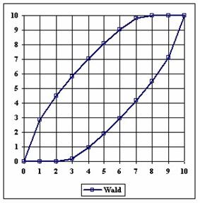
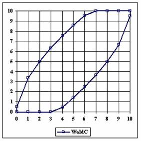
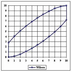
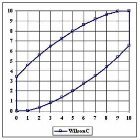
Figure 1. The lower and upper boundaries for proportion at X (0 ≤ X ≤ n) and n = 10
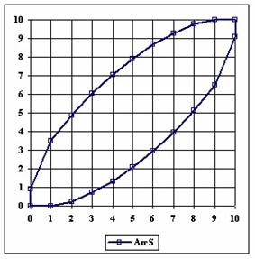
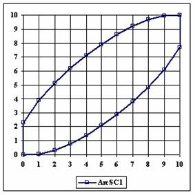
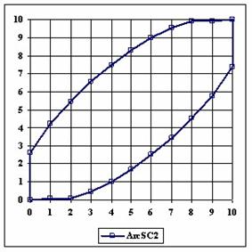
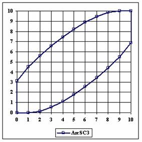
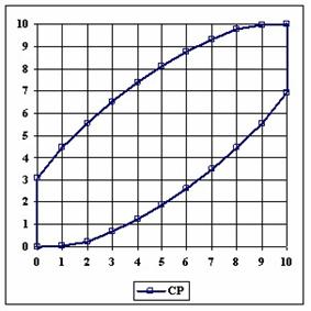
Figure 1. The lower and upper boundaries for proportion at X (0 ≤ X ≤ n) and n = 10
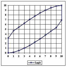
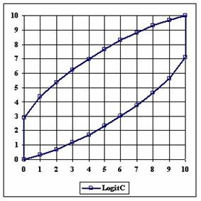
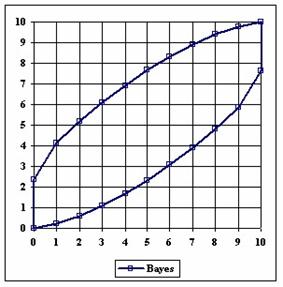
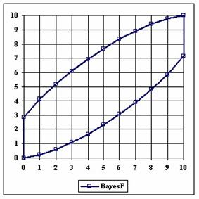
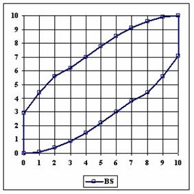
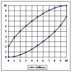
Figure 1. The lower and upper boundaries for proportion at X (0 ≤ X ≤ n) and n = 10
The contour plot using a method based on hypothesis of binomial distribution were graphically represented in figure 2 (graphical representation were created using a PHP program describe in the previous article of the series) [17]. With red color was represented the 0 values, with yellow the 0.5 values and with blue the 1 values. The intermediary color between the couplets colors (red, yellow, and blue) were represents using 18 hues.
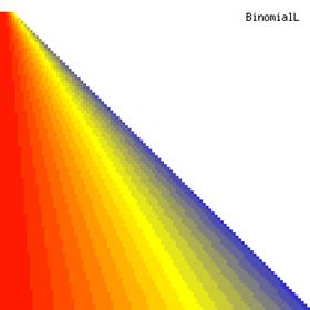
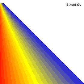
Figure 2. The contour plot for proportion (ci1) and its confidence intervals boundaries (BinomialL and BinomialU) computed with original Binomial method
The percentage of experimental errors depending on selected method and sample size are calculated and compared. The results are below. For a sample size equal with 10, the graphical representations of the experimental errors depending on selected method are in figure 3.
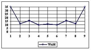
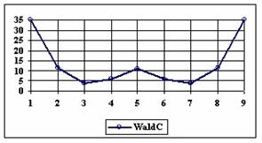
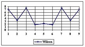
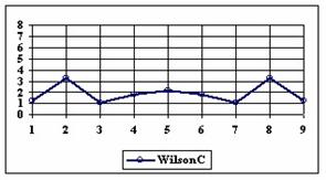
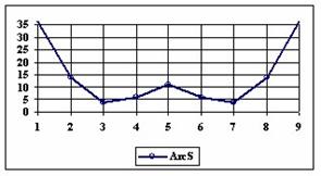
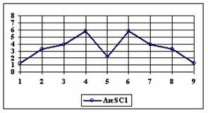
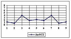
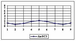
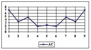
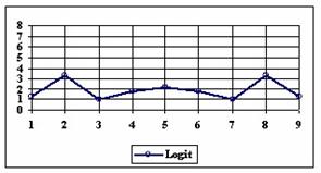
Figure 3. The percentages of the experimental errors for proportion for n=10 depending
on X (0 < X < n)
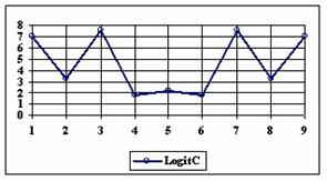
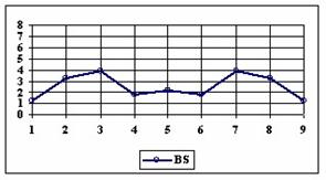
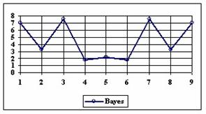


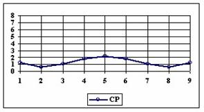
Figure 3. The percentages of the experimental errors for proportion for n=10 depending
on X (0 < X < n)
The graphics of the experimental errors percentages for a sample size of 30 using specified methods are in figure 4.
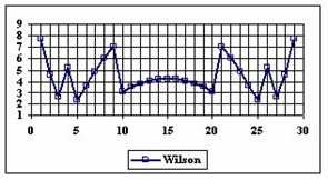
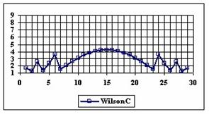
Figure 4. The percentage of the experimental errors for proportion for n = 30
depending on X (0 < X < n)
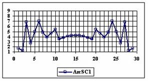
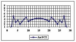
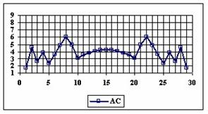
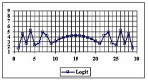
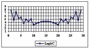
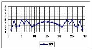
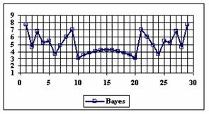
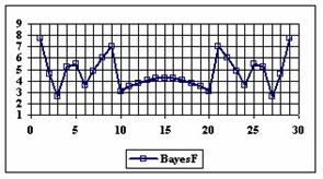
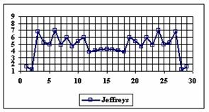
Figure 4. The percentage of the experimental errors for proportion for n = 30
depending on X (0 < X < n)
The graphical representations of the percentage of the experimental errors for a sample size equal with 100 using specified methods are in figure 5.
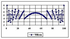

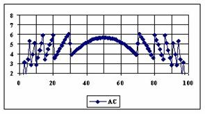
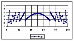
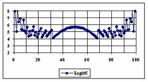
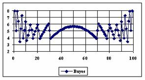
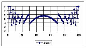
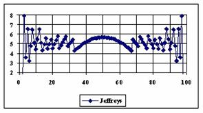
Figure 5. The percentages of the experimental errors for proportion for n = 100
depending on X (0 < X < n)
The diagrams of the experimental errors percentages for a sample size of 300 using specified methods are in figure 6.
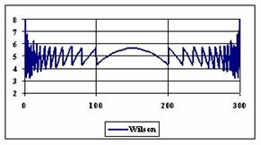
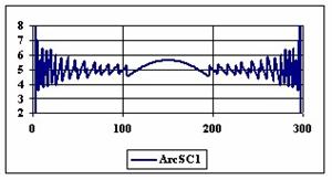
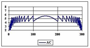
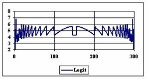
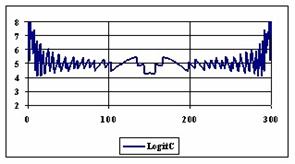
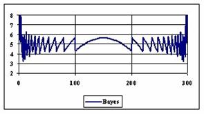
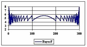
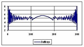
Figure 6. The percentages of the experimental errors for proportion for n = 300
depending on X (0 < X < n)
The methods Logit, LogitC and BayesF obtained the lowest standard deviation of the experimental errors (0.63%).
The graphical representations of the percentage of the experimental errors for a sample size equal with 1000 using specified methods are in figure 7.
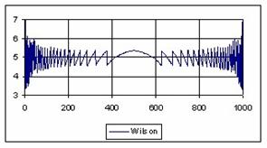
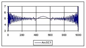
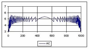
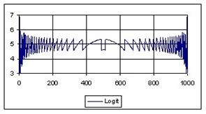
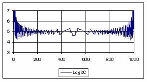
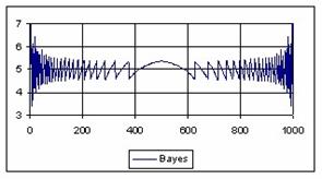
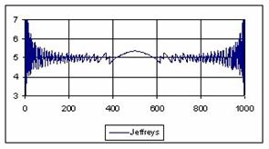
Figure 7. The percentage of the experimental errors fort n = 1000 depending on X (0<X<n)
For n = 1000 the Bayes method (0.39%) obtained the less standard deviations.
Figure 8 contain the subtraction and addition of the experimental standard deviation of the errors from the average of the experimental errors from n=4 to n=100.
Figure 8. The [AM-STDEV, AM+STDEV] range for n = 4 to n = 100 depending on n, where AM is the average and STDEV is the standard deviation of experimental errors
The computed averages and the standard deviations of experimental errors for three ranges of sample sizes (4-10, 11-30, and 30-100), were presented in table 2.
|
n
|
Wilson
|
ArcSC1
|
Logit
|
LogitC
|
BayesF
|
Jeffreys
|
|
4-10
|
5.20 (2.26)
|
2.36 (1.22)
|
3.54 (2.02)
|
4.90 (2.29)
|
4.90 (2.29)
|
5.69 (2.41)
|
|
11-30
|
5.04 (1.93)
|
4.17 (1.74)
|
3.43 (1.19)
|
4.88 (1.66)
|
4.88 (1.88)
|
4.78 (1.58)
|
|
30-100
|
4.98 (1.20)
|
4.76 (1.25)
|
4.39 (1.03)
|
5.07 (1.04)
|
4.94 (1.18)
|
4.92 (1.23)
|
Table 2. The average of the experimental errors and standard deviation
for three ranges of n
The graphical representations of the subtraction and addition of the experimental standard deviation of the errors from the average of the experimental errors from n=101 to n=200 are in figure 9.
Figure 9. The [AM-STDEV, AM+STDEV] range for n = 100 to n = 200 depending on n, where AM is the average and STDEV is the standard deviation of experimental errors
The computed averages of the experimental errors and standard deviations of these errors, for some ranges of sample sizes are in table 3.
|
N
|
Wilson
|
ArcSC1
|
Logit
|
LogitC
|
BayesF
|
Jeffreys
|
|
101-110
|
4.96 (1.00)
|
4.91(1.05)
|
4.64 (0.90)
|
5.10 (0.88)
|
5.02 (0.99)
|
5.04 (1.03)
|
|
111-120
|
4.93 (0.92)
|
4.87 (0.99)
|
4.62 (0.82)
|
5.09 (0.83)
|
4.97 (0.89)
|
4.95 (0.95)
|
|
121-130
|
5.03 (0.93)
|
5.01 (0.99)
|
4.71 (0.87)
|
5.10 (0.84)
|
5.05 (0.88)
|
5.02 (0.96)
|
|
131-140
|
4.94 (0.88)
|
4.86 (0.91)
|
4.62 (0.80)
|
5.03 (0.80)
|
4.96 (0.84)
|
4.91 (0.91)
|
|
141-150
|
5.08 (0.85)
|
4.99 (0.92)
|
4.74 (0.83)
|
5.14 (0.77)
|
5.08 (0.84)
|
5.06 (0.89)
|
|
151-160
|
4.96 (0.86)
|
4.88 (0.90)
|
4.64 (0.80)
|
5.01 (0.79)
|
4.95 (0.84)
|
4.96 (0.87)
|
|
161-170
|
4.90 (0.79)
|
4.95 (0.87)
|
4.73 (0.76)
|
5.09 (0.73)
|
4.96 (0.77)
|
4.97 (0.82)
|
|
171-180
|
4.98 (0.81)
|
5.00 (0.87)
|
4.77 (0.76)
|
5.10 (0.74)
|
5.01 (0.77)
|
5.04 (0.82)
|
|
181-190
|
4.91 (0.78)
|
4.89 (0.81)
|
4.68 (0.70)
|
5.03 (0.73)
|
4.91 (0.75)
|
4.94 (0.79)
|
|
191-200
|
4.97 (0.75)
|
4.94 (0.80)
|
4.78 (0.70)
|
5.14 (0.69)
|
4.98 (0.71)
|
5.01 (0.77)
|
|
101-200
|
4.97 (0.86)
|
4.93 (0.91)
|
4.69 (0.79)
|
5.08 (0.78)
|
4.99 (0.83)
|
4.99 (0.88)
|
|
201-300
|
4.97 (0.69)
|
4.96 (0.73)
|
4.80 (0.65)
|
5.07 (0.66)
|
4.97 (0.67)
|
5.01 (0.71)
|
Table 3. Averages of the experimental error and standard deviation (parenthesis)
for proportion at n = 101 to n = 300
The contour plots of experimental error for each method when the sample size varies from 4 to 103 were illustrated in figure 10. On the contour plots were represented the error from 0% (red color) to 5% (yellow color) and ≥10% (blue color) using 18 hue. The vertical axis represent the values of sample size (n, from 4 to 103) and the horizontal axis the values of X (0 < X < n).


Figure 10. The contour plot of the experimental errors for 3 < n < 104
Figure 10. The contour plot of the experimental errors for 3 < n < 104
Figure 10. The contour plot of the errors for 3 < n < 104
A quantitative expression of the methods can be the deviations of the experimental errors for each proportion relative to the significance level α = 5% (Dev5) for a specified sample size (n), expression which was presented in material and methods section of the paper. The experimental results for n = 4..103, using Wilson, BayesF, Jeffreys, Logit, LogitC and Binomial methods, were taken and were assessed by count the best values of Dev5. The graphical representations of the frequencies are in figure 11.
Figure 11. The best frequencies of deviations of the experimental error relative to the significant level (α = 5%) for n = 4...103
For the random experiment (random values for variable X from 1 to n-1, and random values for sample size n in the range 4
1000, the results are in tables 4-7 and graphical represented in figure 12.
In the figure 12 were represented with black dots the frequencies of the experimental error for each specified method; with green line the best frequencies of the errors interpolation curve with a Gauss curve (dIG(er)); with red line the Gauss curves of the average and standard deviation of the frequencies of the experimental errors (dMV(er)). The Gauss curve of the frequencies of experimental errors deviations relative to the significance level (d5V(er)) was represented with blue squares, and the Gauss curve of the standard binomial distribution of the imposed frequencies of the errors (pN(er, 10)) with black line.
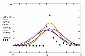
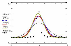
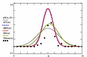
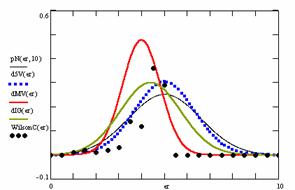
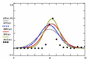
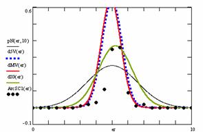

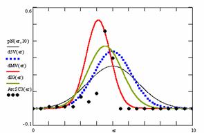
Figure 12. The pN(er, 10), d5V(er), dMV(er), dIG(er) and the frequencies
of the experimental errors for each specified method and random X, n
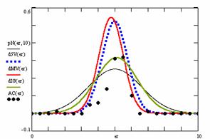
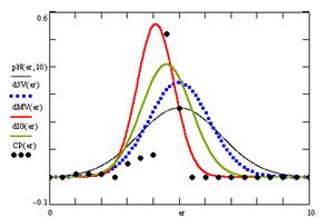

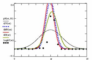
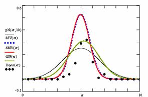
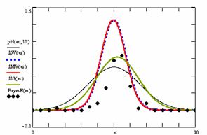
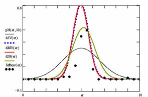
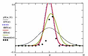
Figure 12. The pN(er, 10), d5V(er), dMV(er), dIG(er) and the frequencies
of the experimental errors for each specified method for random X, n
Table 4 contains the deviations of the experimental errors relative to significance level (Dev5), the absolute differences of the average of experimental errors relative to the imposed significance level (|5-M|), and standard deviations (StdDev). Table 5 contains the absolute differences of the averages that result from Gaussian interpolation curve to the imposed significance level (|5-MInt|), the deviations that result from Gaussian interpolation curve (DevInt), the correlation coefficient of interpolation (r2Int), and the Fisher point estimator (FInt).
|
Nr
|
Method
|
Dev5
|
Method
|
|5-M|
|
Method
|
StdDev
|
|
1
|
Binomial
|
0.61
|
Binomial
|
0.03
|
LogitC
|
0.60
|
|
2
|
LogitC
|
0.62
|
Jeffreys
|
0.03
|
Binomial
|
0.61
|
|
3
|
ArcSC1
|
0.62
|
Bayes
|
0.03
|
ArcSC1
|
0.62
|
|
4
|
Jeffreys
|
0.65
|
BayesF
|
0.03
|
Jeffreys
|
0.65
|
|
5
|
Bayes
|
0.76
|
Wilson
|
0.06
|
CP
|
0.72
|
|
6
|
BayesF
|
0.76
|
ArcSC1
|
0.08
|
AC
|
0.73
|
|
7
|
Wilson
|
0.76
|
WaldC
|
0.12
|
Logit
|
0.74
|
|
8
|
AC
|
0.76
|
LogitC
|
0.14
|
ArcSC2
|
0.74
|
|
9
|
Logit
|
0.77
|
AC
|
0.22
|
Bayes
|
0.76
|
|
10
|
WaldC
|
1.09
|
Logit
|
0.23
|
BayesF
|
0.76
|
|
11
|
CP
|
1.16
|
ArcS
|
0.40
|
Wilson
|
0.76
|
|
12
|
ArcSC3
|
1.17
|
Wald
|
0.72
|
ArcSC3
|
0.76
|
|
13
|
ArcSC2
|
1.18
|
ArcSC3
|
0.89
|
WilsonC
|
0.84
|
|
14
|
ArcS
|
1.30
|
CP
|
0.90
|
WaldC
|
1.08
|
|
15
|
WilsonC
|
1.31
|
ArcSC2
|
0.91
|
ArcS
|
1.23
|
|
16
|
Wald
|
1.84
|
WilsonC
|
1.01
|
Wald
|
1.69
|
Table 4. Methods ordered by performance according to Dev5, |5-M| and StdDev criterions
|
Nr
|
Method
|
|5-MInt|
|
Method
|
DevInt
|
Method
|
r2Int
|
FInt
|
|
1
|
AC
|
0.11
|
LogitC
|
0.82
|
Wald
|
0.62
|
31
|
|
2
|
Logit
|
0.13
|
Binomial
|
0.88
|
WilsonC
|
0.65
|
36
|
|
3
|
WaldC
|
0.14
|
Jeffreys
|
0.95
|
ArcSC3
|
0.66
|
36
|
|
4
|
LogitC
|
0.20
|
WaldC
|
0.97
|
CP
|
0.67
|
38
|
|
5
|
ArcSC1
|
0.22
|
CP
|
0.97
|
ArcSC2
|
0.68
|
40
|
|
6
|
Jeffreys
|
0.22
|
ArcS
|
1.02
|
WaldC
|
0.69
|
42
|
|
7
|
Bayes
|
0.23
|
ArcSC3
|
1.08
|
Wilson
|
0.71
|
47
|
|
8
|
BayesF
|
0.23
|
ArcSC1
|
1.08
|
ArcS
|
0.71
|
47
|
|
9
|
Wilson
|
0.27
|
ArcSC2
|
1.11
|
AC
|
0.71
|
47
|
|
10
|
Binomial
|
0.27
|
Wald
|
1.25
|
Logit
|
0.71
|
47
|
|
11
|
ArcS
|
0.38
|
AC
|
1.26
|
Bayes
|
0.71
|
47
|
|
12
|
ArcSC3
|
0.47
|
Logit
|
1.27
|
BayesF
|
0.71
|
47
|
|
13
|
ArcSC2
|
0.48
|
Wilson
|
1.27
|
ArcSC1
|
0.72
|
50
|
|
14
|
CP
|
0.49
|
Bayes
|
1.29
|
Jeffreys
|
0.74
|
54
|
|
15
|
Wald
|
0.51
|
BayesF
|
1.29
|
Binomial
|
0.75
|
57
|
|
16
|
WilsonC
|
0.60
|
WilsonC
|
1.33
|
LogitC
|
0.76
|
59
|
Table 5. The methods ordered by |5-Mint|, DevInt, r2Int and FInt criterions
The superposition between the standard binomial distribution curve and interpolation curve (pNIG), the standard binomial distribution curve and the experimental error distribution curve (pNMV), and the standard binomial distribution curve and the error distribution curve around significance level (pN5V) are in table 6.
|
Nr
|
Method
|
pNIG
|
Method
|
pNMV
|
Method
|
pN5V
|
|
1
|
LogitC
|
0.69
|
CP
|
0.56
|
Binomial
|
0.57
|
|
2
|
Binomial
|
0.72
|
LogitC
|
0.56
|
LogitC
|
0.58
|
|
3
|
CP
|
0.74
|
ArcSC2
|
0.57
|
ArcSC1
|
0.58
|
|
4
|
Jeffreys
|
0.75
|
Binomial
|
0.57
|
Jeffreys
|
0.60
|
|
5
|
WaldC
|
0.77
|
ArcSC1
|
0.57
|
Bayes
|
0.66
|
|
6
|
ArcS
|
0.77
|
ArcSC3
|
0.58
|
BayesF
|
0.66
|
|
7
|
ArcSC3
|
0.78
|
WilsonC
|
0.59
|
Wilson
|
0.66
|
|
8
|
ArcSC2
|
0.79
|
Jeffreys
|
0.60
|
AC
|
0.66
|
|
9
|
ArcSC1
|
0.81
|
AC
|
0.64
|
Logit
|
0.67
|
|
10
|
WilsonC
|
0.82
|
Logit
|
0.64
|
WaldC
|
0.82
|
|
11
|
Wald
|
0.83
|
Bayes
|
0.66
|
CP
|
0.85
|
|
12
|
Wilson
|
0.88
|
BayesF
|
0.66
|
ArcSC2
|
0.86
|
|
13
|
Bayes
|
0.88
|
Wilson
|
0.66
|
ArcSC3
|
0.86
|
|
14
|
BayesF
|
0.88
|
WaldC
|
0.82
|
ArcS
|
0.90
|
|
15
|
AC
|
0.89
|
Wald
|
0.82
|
WilsonC
|
0.91
|
|
16
|
Logit
|
0.89
|
ArcS
|
0.84
|
Wald
|
0.93
|
Table 6. Methods ordered by the pNING, pNMV, and pN5V criterions
|
Nr
|
Method
|
pIGMV
|
Method
|
pIG5V
|
Method
|
pMV5V
|
|
1
|
WaldC
|
0.95
|
WaldC
|
0.93
|
Bayes
|
0.99
|
|
2
|
ArcS
|
0.91
|
ArcS
|
0.84
|
BayesF
|
0.99
|
|
3
|
Wald
|
0.85
|
LogitC
|
0.83
|
Binomial
|
0.98
|
|
4
|
Binomial
|
0.79
|
ArcSC2
|
0.83
|
Jeffreys
|
0.98
|
|
5
|
Jeffreys
|
0.79
|
ArcSC3
|
0.83
|
Wilson
|
0.97
|
|
6
|
LogitC
|
0.77
|
WilsonC
|
0.82
|
WaldC
|
0.96
|
|
7
|
CP
|
0.77
|
CP
|
0.81
|
ArcSC1
|
0.95
|
|
8
|
ArcSC3
|
0.77
|
Jeffreys
|
0.80
|
LogitC
|
0.91
|
|
9
|
ArcSC2
|
0.75
|
Wald
|
0.78
|
AC
|
0.88
|
|
10
|
Wilson
|
0.75
|
Binomial
|
0.78
|
Logit
|
0.88
|
|
11
|
WilsonC
|
0.75
|
Logit
|
0.76
|
ArcS
|
0.87
|
|
12
|
Bayes
|
0.73
|
AC
|
0.76
|
Wald
|
0.83
|
|
13
|
BayesF
|
0.73
|
Wilson
|
0.74
|
ArcSC3
|
0.61
|
|
14
|
AC
|
0.72
|
Bayes
|
0.74
|
WilsonC
|
0.60
|
|
15
|
Logit
|
0.72
|
BayesF
|
0.74
|
ArcSC2
|
0.60
|
|
16
|
ArcSC1
|
0.71
|
ArcSC1
|
0.73
|
CP
|
0.59
|
Table 7. The confidence intervals methods ordered by the
pIGMV, pIG5V, and pMV5V criterions
The table 7 contains the percentages of superposition between interpolation Gauss curve and the Gauss curve of error around experimental mean (pIGMV), between the interpolation Gauss curve and the Gauss curve of error around imposed mean (α = 5%) (pIG5V) and between the Gauss curve experimental error around experimental mean, and the error Gauss curve around imposed mean α = 5% (pMV5V).
Discussions
The Wald method (figure 1) provides most significant differences in computing confidence intervals boundaries. If we exclude from discussion the Wald method and its continuity correction method (WaldCI method) we cannot say that there were significant differences between the methods presented; the graphical representation of confidence intervals boundaries were not useful in assessment of the methods.
As a remark, based on the figure 1, for n=10 there were five methods which systematically obtain the average of the experimental errors less then the imposed significant level (α = 5%): WilsonC (1.89%), ArcSC2 and ArcSC3 (1.93% for ArcSC2 and 1.31% for ArcSC2), Logit (1.89%), BS (2.52%) and CP (1.31%). For n = 10 the methods Wilson, LogitC, Bayes and BayesF obtained identical average of experimental errors (equal with 4.61%). We can not accept the experimental errors of Wald, WaldC, ArcS (the average of the experimental errors greater than imposed significant level α = 5%, respectively 17.33%, 13.69% and 15.53%); the ArcSC3 and the CP methods were obtained an average of the experimental errors equal with 1.31%. From the next experiments were excluded the specified above methods.
Looking at the graphical representations from figure 1 and 2, the upper confidence boundaries are the mirror image of the lower confidence boundaries.
For n = 30 the percentages of the experimental errors for the WilsonC (2.77%), ArcSC2 (3.27%) and BS (3.61%) methods were systematically less then the choused significant level (figure 4).
For n = 100 the Logit method obtain experimental errors greater than the imposed significant level of 5% (5.07% at X = 2, 6.43% at X = 4, and so on until X = 29), even if the error mean was less than 5% (4.71%). If we were looked at the average of the experimental errors and of standard deviations of them, the best mean were obtained by: Jeffreys (5.03%), ArcSC1 (4.96%), Wilson (5.07%) and BayesF (5.08%), and the best standard deviation by the methods: LogitC (0.83%), BayesF (0.91%), Logit (0.94%) and Bayes (0.95%).
Analyzing the percentage of the experimental errors for n=300, as we can saw from the graphical representation (figure 6) it result that the Wilson (5.03%), BayesF (5.04%) and ArcSC1 (5.06%) obtained the best average of the experimental errors.
For n = 1000 Wilson (5%), BayesF (5.01%) and ArcSC1(5.01%) obtained the best error mean (5.01%) and BayesF (0.37%) followed by Wilson, ArcSC1, Logit, LogitC.
Looking at the experimental results which present the average and the standard deviations of experimental errors for three specified ranges of sample sizes (see table 2) we remarked that Wilson had the most appropriate average of the experimental errors from the imposed significance level (α = 5%), and in the same time, the smallest standard deviation for n ≤ 10. For 10 < n ≤ 100 the best performance were obtained by the LogitC method.
For values of the samples size varying into the range 101 ≤ n < 201, cannot be observed any differences between Wilson, ArcSC1, Logit, LogitC, BayesF methods if we looked at the graphical representation (figure 9). Even if the graphical representation cannot observe the differences, these differences were real (see table 3). Analyzing the results from the table 3 we observed the constantly performance obtained by BayesF, with just two exceptions its average and standard deviations of the experimental errors were between the first three values. The LogitC method was the most conservative method if we looked at standard deviation, obtaining the first performance in 8 cases from 10 possible at n = 101 to n = 200. If we looked at the average of the errors, it were a little bit hard to decide which was the best, because ArcSC1, LogitC, BayesF and Jeffreys obtained at least two times the best performance reported to the choused significant level (α = 5%). Generally, if we looked at all interval (n = 101..300) it result that Jeffreys (4.991%) obtained the best error mean, followed by BayesF (4.989%).
Analyzing the deviation relative to the imposed significance level for each proportion for a specified sample size (n) (figure 11) some aspects are disclosure. The first observation was that the original method Binomial improved the BayesF and the Jeffreys methods even if, to the limit, the Binomial overlap on BayesF and Jeffreys (see the Binomial method formula):
 ,
, 
The second observation was that the Binomial method obtained the best performance (with 58 apparitions, followed by LogitC with 27 apparitions).
The third observation which can be observed from the experimental data (cannot been seen from the graphical representation) was that for n > 30 Binomial was systematically the method with the best performance (had 54 apparition, followed by LogitC with 13; no apparition for other methods). Even more, starting with n = 67 and until n = 103 the Binomial method obtained every time the best deviations relative to the imposed significance level α = 5%. In order to confirm the hypothesis that for n ≥ 67 the Binomial method obtains the lowest deviations relative to the imposed significance level, the Dev5 for six sample sizes, from n = 104 to n = 109, were computed. For n=104 the Binomial method obtained the lowest deviations relative to the imposed significance level of the experimental errors (0.83, comparing with 0.90 obtained by the LogitC method, and BayesF method with 1.03, and Jefferys with 10.8). This characteristics was obtained systematically (0.76 for n=105, 0.77 for n=106, 0.76 for n=107, 0.75 for n=108, 0.75 for n=109). The observation described above confirm the hypothesis that Binomial method obtained the smallest deviations relative to the significance level α = 5%.
The best three methods reported in specialty literature that obtain the greatest performance in our experiments are in table 8.
|
n
|
Method
|
|
4-10
|
Wilson, LogitC, BayesF
|
|
11-30
|
LogitC, BayesF, Wilson
|
|
31-100
|
LogitC, BayesF, Wilson
|
|
101-300
|
BayesF, LogitC, Wilson
|
Table 8. The best three methods depending on n
Looking at the results obtained from the random samples (X, n random numbers, n range 4..1000 and X range 1..n-1), it can be remarked that the Binomial method obtain the closed experimental error mean to the imposed mean (α = 5%). The LogitC method obtains the lowest standard deviations of the experimental errors (table 4).
The Agresti-Coull was the method which obtained the closed interpolation mean to the imposed mean (table 5), followed by the Logit method; LogitC (closely followed by the Binomial method) was the method with the lowest interpolation standard deviation. The LogitC method followed by the Binomial method provides the best correlation between theoretical curve and experimental data.
It can observed analyzing the results presented in the table 6, that the Logit and the Agresti-Coull methods, followed by the Bayes, BayesF and Wilson were the methods that presented the maximum superposition between the curve of interpolation and the curve of standard binomial distribution. With ArcS method obtains the maximum superposition between the curve of standard binomial distribution and the curve of experimental errors.
The maximum superposition between the Gauss curve of interpolation and the Gauss curve of errors around experimental mean is obtain by the WaldC method, followed by the ArcS, the Wald and the Binomial methods (table 7). The WaldC method obtained the maximum superposition between the Gauss curve of interpolation and the Gauss curve of errors around imposed mean.
The Bayes and the BayesF methods obtained the maximum superposition between experimental error Gauss curve distribution and the error Gauss curve distribution around imposed mean.
Conclusions
Choosing a specified method of computing the confidence intervals for a binomial proportion depend on an explicit decision whether to obtain an average of the experimental errors closed to the imposed significance level or to obtain the lowest standard deviation of the errors for a specific sample size.
In assess of the confidence intervals for a binomial proportion, the Logit and the Jeffreys methods obtain the lowest deviations of experimental errors relative to the imposed significance level and the average of the experimental errors smaller than the imposed significance level. Thus, if we look after a confidence intervals which to assure the lowest standard deviation of the errors we will choose one of these two methods.
If we want a method which to assure an average of the experimental error close to the imposed significance level, then the BayesF method could be choose for a sample size on the range 4 ≤ n ≤ 300.
The Binomial method obtains the best performance in confidence intervals estimation for proportions using random sample size from 4 to 1000 and random binomial variable from 1 to n-1 and systematically obtains the best overall performance starting with a sample size greater than 66.
Acknowledgements
First author is thankful for useful suggestions and all software implementation to Ph. D. Sci., M. Sc. Eng. Lorentz JÄNTSCHI from Technical University of Cluj-Napoca.
References
[1]. Achimaş Cadariu A., Diagnostic Procedure Assessment Chapter from Achimaş Cadariu A. Scientific Medical Research Methodology, Medical University Iuliu Haţieganu Publishing House, Cluj-Napoca, 1999, p. 29-38 (in Romanian).
[2]. Hamm R. M., Clinical Decision Making Spreadesheet Calculator, University of Oklahoma Health Sciences Center, available at:www.emory.edu/WHSC/MED/EMAC/curriculum/diagnosis/oklahomaLRs.xls
[3]. Epidemiology&Lab Statistics from Study Counts, EpiMax Table Calculator, Princeton, New Jersey, USA, available at: http://www.healthstrategy.com/epiperl/epiperl.htm
[4]. Achimaş Cadariu A., Evidence Based Gastroenterology Chapter from Grigorescu M. Treaty of Gastroenterology, Medical National Publishing House, Bucharest, 2001, p. 629-659 (in Romanian).
[5]. Sackett D., Straus E.S., Richardson W.S., Rosenberg W., Haynes R.B., Therapy Chapter in Evidence-based Medicine: How to Practice and Teach EBM, 2nd ed. Edinburgh, Churchill Livingstone, 2000, p. 105-154.
[6]. Drugan T., Bolboacă S., Colosi H., Achimaş Cadariu A., Ţigan Ş., Dignifying of prognostic and Risk Factors Chapter in Statistical Inference of Medical Data, ALMA MATER Cluj-Napoca, 2003, p. 66-71 (in Romanian).
[7]. Newcombe R.G., Two-sided confidence intervals for the single proportion; comparison of several methods, Statistics in Medicine, 1998, 17, p. 857872.
[8]. Rothman K., Modern Epidemiology, Little Brown, Boston, 1986, p. 121.
[9]. Rosner B., Hypothesis Testing: Categorical Data Chapter in Fundamentals of Biostatistics, Forth Edition, Duxbury Press, Belmont, 1995, p. 345-442.
[10]. Brown D.L., Cai T.T., DasGupta A., Interval estimation for a binomial proportion, Statistical Science, 2001, 16, p. 101-133.
[11]. Blyth C.R., Still H.A., Binomial confidence intervals, J. Amer. Stat. Assoc. 1983, 78, p. 108-116.
[12]. Michael D., Edwardes B., The Evaluation of Confidence Sets with Application to Binomial Intervals, Statistica Sinica, 1998, 8, p. 393-409.
[13]. Santner T.J., A note on teaching binomial confidence intervals, Teaching Statistics, 1998, 20, p. 20-23.
[14]. Vollset S.E., Confidence intervals for a binomial proportion, Statistics in Medicine, 1993, 12, p. 809-824.
[15]. Agresti A., Coull D.A., Approximate is better then exact for interval estimation of binomial proportion. Amer. Statist. 1998, 52, p. 119-126.
[16]. Drugan T., Bolboacă S., Jäntschi L., Achimaş Cadariu A., Binomial Distribution Sample Confidence Intervals Estimation 1. Sampling and Medical Key Parameters Calculation, Leonardo Electronic Journal of Practices and Technologies, 2003, 3, p. 45-74.
[17]. Pires M.A., Confidence intervals for a binomial proportion: comparison of methods and software evaluation, available at: http://www.math.ist.utl.pt/~apires/AP_COMPSTAT02.pdf
[18]. Blyth R.C., Approximate Binomial Confidence Limits, Journal of the American Statistical Association, 1986, 81, p. 843-855.
[19]. Casella G., Berger R.L., Statistical Inference, Wadsworth&Brooks/Cole, Belmont, CA., 1990.
Issue 03, p. 111-117
Comparative Study of Monolayer Fatty Acids at the Air/Water Interface
Bianca Monica RUS
Technical University of Cluj-Napoca, Romania
Abstract
The behavior of insoluble monolayer of surfactants spread at the air/water interfaces is frequently studied by recording compression isotherms.The compression isotherms given in terms of surface pressure versus mean molecular area are well reproducible for a chosen spreading molecular area of fatty acids, like stearic acid, oleic acid and linoleic acid.
Mathematical modeling of these isotherms is performed by means of surface state equations. In the literature, a great variety of such equations have been proposed. In the present paper is made a study of the compression isotherms of oleic acid (OA) monolayer spread at the air /water interface on acidic aqueous solutions (pH = 2).
Keywords
Fatty Acid Monolayer, Equations of State, Air/water Interface
I. Introduction
The thermodynamic and structural characterization of fatty acid films at the air-water interface has received a remarkable attention over the past several decades [1-6]. The thermodynamic analysis of compression isotherms in terms of surface pressure (π, mN/m) versus mean molecular area (A, nm2/molecule) leads to equations of state that describes well the phase behavior of fatty acid monolayer.
At very low surface pressures, monolayer might be considered to behave like two-dimensional gases. Therefore, in these conditions, the validity of the two-dimensional perfect gas state equation [4]:
πA = kT (1)
may be expected, where k is Boltzmanns constant and T is the absolute temperature. Due to the experimental difficulties in measuring very low surface pressures, this region is less investigated.
Much more data are available in the range of 0.2 mN/m < π <10 mN/m, where monolayer generally are in a liquid expanded state. Since the cross-sectional area of the surfactant molecules cannot be neglected and it represents a mean area necessity named also co-area, in equation (1) the A value has been corrected for a co-area (A0), obtaining [9]:
π(A - A0) = kT (2)
where A0 is frequently taken as an adjusted parameter.
Since in the liquid state the intermolecular interactions might be more important than the own molecular area of the surfactant, an internal pressure, π0, can be introduced. Correcting π in equation (1) for this internal pressure, one obtains:
(π+π0)A = kT (3)
By taking into account both intermolecular attractive forces and the above mentioned co-area, the state equation (1) becomes [10]:
(π +π0)(A - A0) = kT (4)
Further, a two-dimensional state equation, analogous with the Van der Waals equation:
(π + α/A2)(A - A0) = kT (5)
has also been proposed. Equation (5) results from equation (4), by taking π0 = α/A2 on the base of the same reason, which in the case of a bulk gaseous phase leads to the presumption that the three-dimensional internal pressure is inversely proportional with the square of the volume.
There were made several attempts to correlate the parameter α with molecular structure and with intermolecular interactions. On the basis of the scaled particle theory for fatty acids the state equation:
(π +α/A2)[A (1 A0'/A)2] = kT (6)
was derived [11]. In this equation A0' = πd2/4 represents the area of a hard disc having its diameter equal to d, which is thought to be equivalent with the cross-sectional area of the saturated hydrocarbon chain. The correlation between A0' and the co-area A0 is A0'=A0/2. The parameter α was also correlated with molecular and intermolecular characteristics.
For cohering uncharged films the equation:
(π + α/A3/2) (A - A0) = kT (7)
was derived [12] and it was found to be in good agreement with some experimental results.
According to the duplex film model, a surfactant monolayer spread at the air/water interface may be considered as a monolayer solution formed of the surfactant head groups dissolved in water and having the theoretical surface pressure πh, covered by an oily layer consisting of the hydrophobic chains of surfactant molecules. Denoting by (-π0) the spreading coefficient of this oil on the hypothetical surface solution of surfactant head groups and interfacial water, the overall surface pressure may be expressed as:
π = -π0 + πh (8)
By considering an insoluble monolayer, on the basis of the equality of the chemical potential of water in the bulk subphase and in the monolayer solution of headgroups, πh may be given by a Butler type equation [13]:
 (9)
(9)
where, A1, a1, γ1 and x1 stands for the molecular area, activity, activity coefficient and molar fraction of water molecules in the monolayer solution, respectively. Combination of equation (8) and (9) yields [14]:
 (10)
(10)
By considering the headgroup monolayer to be a binary regular solution, one has
 (11)
(11)
where β12 and x2 stands for the interaction parameter between the polar head group and water molecules in the monolayer and for the molar fraction of the head groups in the monolayer, respectively.
Finally, the following equation of state is obtained:
 (12)
(12)
It is well to mention that other state equations have also been derived based on statistical considerations of the conformation of hydrocarbon chain segments [15, 16].
In the present paper is made a study of the compression isotherms of oleic acid (OA) monolayer spread at the air /water interface on acidic aqueous solutions (pH = 2).
II. Material and Methods
In view of testing the state equations the OA monolayer has been chosen as model system. The compression isotherm recorded on a subphase with pH = 2 has been used since at this pH the protolytic equilibrium in the monolayer is shifted practically completely towards the neutral OA molecules [7]. The experimental π vs. A curve is given in fig.1 (curve 1). The theoretical curve, corresponding to equation (1) is visualized in the same figure (curve 2). As seen, at high A values important deviations from the perfect behavior appear in the negative direction, indicating the role of the intermolecular attractive forces. On the contrary, at lower A values, the deviations become positive.
III. Results and Discussion
The other state equations contain single (equations (2) and (3) or even two equations 4-7) parameters to be derived from experimental data. Since a good mathematical description of the compression isotherms by means of state equations can be expected in the case of expanded films, i.e. at low surface pressures, the π ≤ 7 mN/m has been chosen. This domain is delimited in Fig. 1 by dashed straight lines, and we had in this region a number of 17 experimental points, i.e. Ai - πi pairs. These data were processed following a curve fitting method. For this purpose, the standard deviation □ of the experimental points from the theoretical ones was calculated and minimized by performing a systematic variation of the parameter / parameters to be derived.
Fig. 1. πvs. A isotherms for OA monolayer. Experimental curve(1); theoretical curves (2-5) calculated by using parameters given in Table 1 and state equations: curve (2) equation (1); (3) - equation (2); (4) - equations (3); (5) - equation (4).
In the case of equation (2) and (3), by varying A0 and π0, respectively, the minimum standard deviation, m, was determined, which is given in Table 1, together with the corresponding parameter value. By using the latters the theoretical ones, given in Fig. 1, were calculated (curves 3 and 4). As seen, equation (2) gives a rather unrealistic, negative A0 value, while equation (3) yields a π0 value corresponding to intermolecular attraction. Neither equation (2), nor equation (3) is able to give a good description of the experimental curve, the m value being rather high.
By using equations with two adjustable parameters, a double minimization of □ is to be performed. To this end, one of the parameters is maintained at a constant value, and by varying the other one, the minimum of □, denoted as □m is determined. The systematic variation of the first parameter allows us to determine the minimum of the □m values, (□m)m, indicating the best values of both parameters to be derived. These double minimum values of ∆ are given in Table 1, and the theoretical curve calculated by means of equation (4), using π0 and A0 values given in Table 1, is also visualized in Fig. 1, curve (5). Obviously, the use of two adjustable parameters entails a spectacular improvement of the approximation.
Table 1. Parameters of the state equation and standard deviations derived for OA monolayer (π ≤ 7 mN/m)
|
Eq
|
π0 (mN/m)
|
A0 (nm2/molec)
|
α*
|
β12∙1020 (Nm)
|
□** (mN/M)
|
|
(1)
|
-
|
-
|
-
|
-
|
6.09
|
|
(2)
|
-
|
-1.123
|
-
|
-
|
1.95
|
|
(3)
|
6.0
|
-
|
-
|
-
|
1.19
|
|
(4)
|
10.5
|
0.169
|
-
|
-
|
0.29
|
|
(6)
|
-
|
0.268
|
5.691
|
-
|
0.17
|
|
(7)
|
10.46
|
-
|
-
|
-0.08
|
0.29
|
|
(9)
|
-
|
-
|
0.842
|
-1.07
|
0.15
|
|
(10)
|
-
|
-
|
8.601
|
-2.28
|
0.09
|
|
(11)
|
-
|
-
|
1.153
|
-5.73
|
0.13
|
*Units: 1) 10-30 Nm2; 2) 10 -20 Nm; 3) 10-38 Nm2; in all cases per molecule
**It means m in the case of equations (2) and (3), and (m)m with equations (4), (6), (7) and (9-11).
As seen from Table 1, equation (6) gives better results than the others. As far as equation (7) is concerned, its use raises several problems, related to calculation of the molar fractions in the monolayer.
References
1. Dynarowicz-Latka P., Dhanabalan A., Oliveira O. N., Colloid and Interface Sci., 91 (2), 2001, p. 221-293.
2. Harkins W. D., The Physical Chemistry of Surface Films, Reinhold, New York, 1952.
3. Davies J.T., and Rideal, E.K., Interfacial Phenomena, Academic Press, New York, 1963.
4. Gaines G.L.Jr., Insoluble Monolayers at Liquid-Gas Interface, Wiley-InterScience, New York, 1966.
5. Hiemenz P.C., Principles of Colloid and Surface Chemistry, Dekker, New York, 1966.
6. Lim Y.C., and Berg J.C., J. Colloid and Interface Sci., 51 (1), 1975, p. 162.
7. Tomoaia Cotisel M., Zsako J., Mocanu A., Lupea M., Chifu E., J. Colloid Interface Sci., 117, 1987, p. 464.
8. Tomoaia-Cotisel M., Mocanu A., Pop V.D, Plesa D., Plesa S., Albu I., Equations of State for Films of Fatty Acids at the Air/Water Interface, The VIIth Symposium of Colloid and Surface Chemistry, Bucharest, 2002.
9. Volmer M., Z. Physik. Chem., 115, 1925, p. 253.
10. Langmuir I., J. Chem. Phys., 1 , 1933, p. 756.
11. Reiss H., Frisch H.L., Lebowitz J.L., J. Chem. Phys., 31, 1959, p. 369.
12. Guastalla J., Cahiers Phys., 10, 1942, p. 30 ; J. Chem. Phys., 43, 1946, p. 184.
13. Butler J.A.V., Proc. Royal. Soc. London, Ser. A, 135, 1932, p. 348.
14. Lim Y.C., Berg J.C., J. Colloid Interface Sci., 51, 1975, p. 162.
15. Motomura K., Motomura R., J. Colloid Interface Sci., 29, 1969, p. 617.
16. MacDowell L.G., Vega C., Sanz E., J. Chem. Phys., 115 (13), 2001, p. 6220.