Binomial Distribution Sample Confidence Intervals Estimation
6. Excess Risk
Sorana BOLBOACĂ, Andrei ACHIMAŞ CADARIU
“Iuliu Haţieganu” University of Medicine and Pharmacy, Cluj-Napoca, Romania
Abstract
We present the problem of the confidence interval estimation for excess risk (Y/n-X/m fraction), a parameter which allows evaluating of the specificity of an association between predisposing or causal factors and disease in medical studies. The parameter is computes based on 2x2 contingency table and qualitative variables. The aim of this paper is to introduce four new methods of computing confidence intervals for excess risk called DAC, DAs, DAsC, DBinomial, and DBinomialC and to compare theirs performance with the asymptotic method called here DWald.
In order to assess the methods, we use the PHP programming language and a PHP program was creates. The performance of each method for different sample sizes and different values of binomial variables were assess using a set of criterions. First, the upper and lower boundaries for a given X, Y and a specified sample size for choused methods were compute. Second, were assessed the average and standard deviation of the experimental errors, and the deviation relative to imposed significance level α = 5%. Four methods were assessed on random numbers for binomial variables and for sample sizes from 4 to 1000 domain.
The experiments show that the DAC methods obtain performances in confidence intervals estimation for excess risk.
Keywords
Confidence interval estimation; Excess risk; Risk factors assessments
Introduction
Evaluation of the specificity of an association between predisposing or causal factors and disease can be express as excess risk. The excess of risk is define as: "the differences between individual risk on exposure group and individual risk on nonexposure group"[1], [2]. In order to evaluate de specificity of association between predisposing or causal factors and disease a point estimation of excess risk with its confidence intervals are very useful.
The confidence intervals for differences between two proportions were described in a few papers [3], [4], [5], [6]. In the literature there were not differentiated described the absolute and the relative differences between two proportion. Newcombe [3] recommend two methods based on Wilson method described at proportions [7] as the best method to the difference between two proportions.
The aim of this paper is to introduce four new methods of computing confidence intervals for excess risk called DAC, DAs, DAsC, DBinomial, and DBinomialC and to compare theirs performance with the asymptotic method called here DWald.
Materials and Methods
Excess risk can be compute based on 2´2 contingency table where four groups of cases can be defining: real positive cases (patients with diseases and expose to the risk factor), usually noted with a, false positive cases (patients which do not present the disease but have a exposure to the risk factor), usually noted here with b. The false negative cases (patients that present the disease but was not exposed to the risk factor), usually noted with c and true negative cases (patient which do not present the disease and were not expose to the risk factor), noted usually with d.
Using the definition of the excess risk and the next substitution on 2´2 contingency table: a = Y, b = n-Y, c = X, d = m-X (X and Y are independent binomial distribution variables of sizes m and n) the excess risk (ER) become:
![]() (1)
(1)
Mathematically speaking, the excess risk function is a Y/n-X/m type function and noted with ci5 in our program [7].
Based on the classically definition of confidence intervals introduce at proportion [8] were defined six functions: DWald, DAC, DAs, DAsC, DBinomial, and DBinomailC:
 (2)
(2)
 (3)
(3)
 (4)
(4)
 (5)
(5)
![]() (6)
(6)
 (7)
(7)
where D function computes the differences of two confidence intervals by the formula:
![]() (8)
(8)
The DWald is the standard method take from the literature. The DAC,
DAs, DAsC, DBinomial and DBinomialC methods are new implemented
methods based on the corresponding methods used for estimating one-proportion.
The DAC method was obtained by introducing an adjustment parameter
represented by the![]() for binomial variables (X, Y) and
for binomial variables (X, Y) and ![]() for sample
sizes (m, n), adjustment introduce by the Agresti and Coull to the
one-dimensional confidence interval expression (CI = CI(X,n)) [9].
The DAs method based on the ArcS method described at proportion
and adapted for differences between two proportions. The continuity corrected
method (DAsC) used the adjustment parameters
for sample
sizes (m, n), adjustment introduce by the Agresti and Coull to the
one-dimensional confidence interval expression (CI = CI(X,n)) [9].
The DAs method based on the ArcS method described at proportion
and adapted for differences between two proportions. The continuity corrected
method (DAsC) used the adjustment parameters ![]() and respectively
and respectively![]() , parameters, deduced
experimental. The DBinomial and DBinomialC methods based on the
original method, Binomial, method used for the first time in confidence
interval estimation of a proportion [7].
, parameters, deduced
experimental. The DBinomial and DBinomialC methods based on the
original method, Binomial, method used for the first time in confidence
interval estimation of a proportion [7].
The described methods of computing confidence intervals for excess risk are implements in a PHP program. The source codes for methods are:
function DWald($X,$m,$Y,$n,$z,$a){
$ad = $Y/$n-$X/$m;
$t0 = $z * pow($X*($m-$X)/pow($m,3)+$Y*($n-$Y)/pow($n,3),0.5);
$tXi = $ad-$t0; if($tXi<-1) $tXi=-1;
$tXs = $ad+$t0; if($tXs>1) $tXs=1;
return array( $tXi , $tXs ); }
function DAC($X,$m,$Y,$n,$z,$a){
return DWald($X+pow($z,2)/4/pow(2,0.5),$m+pow($z,2)/2/pow(2,0.5),
$Y+pow($z,2)/4/pow(2,0.5),$n+pow($z,2)/2/pow(2,0.5),$z,$a);}
function DAs($X,$m,$Y,$n,$z,$a){
$ad = $Y/$n-$X/$m;
$t0 = $z * pow($X*($m-$X)/pow($m,3)+$Y*($n-$Y)/pow($n,3)+
+asin(pow($ad,0.5))/($m*$n), 0.5);
$tXi = $ad-$t0; if($tXi<-1) $tXi=-1;
$tXs = $ad+$t0; if($tXs>1) $tXs=1;
return array( $tXi , $tXs ); }
function DAsC($X,$m,$Y,$n,$z,$a){
$ad = $Y/$n-$X/$m;
$t0 = $z * pow($X*($m-$X)/pow($m,3)+$Y*($n-$Y)/pow($n,3)
+asin(pow($ad,0.5))/($m*$n)/2+0.25/pow($m,3)+0.25/pow($n,3),0.5);
$tXi = $ad-$t0; if($tXi<-1) $tXi=-1;
$tXs = $ad+$t0; if($tXs>1) $tXs=1;
return array( $tXi , $tXs ); }
function DBinomial($X,$m,$Y,$n,$z,$a){
return D("Binomial",$X,$m,$Y,$n,$z,pow($a/2,0.5),pow($a/2,0.5));}
function DBinomialC($X,$m,$Y,$n,$z,$a){ return
D("Binomial",$X,$m,$Y,$n,$z,pow($a/2,0.5)/(1-1/log($m)/8),pow($a/2,0.5)/(1-1/log($n)/8));}
In order to obtain a 100·(1-α) = 95% confidence intervals (is most frequently used confidence intervals) the experiments were runs at a significance level α = 5% (noted with a in our program). Corresponding to choused significance level was used its normal distribution percentile z1-α/2 = 1.96 (noted with z in our program). The sequence of the program is:
define("z",1.96); define("a",0.05);
The performance of each method for different sample sizes (m, n) and different values of binomial variables (X, Y) was compares using a set of criterions.
First were computed and graphical represented the lower and upper confidence intervals limits for equal sample sizes (m = n = 50) using the DBinomial and the DAC methods:
$c_i=array("DBinomialC","DAC");
define("N_min",50); define("N_max",51); est_ci2_er(z,a,$c_i,"ci5","ci");
Second, were analyzed the experimental errors and standard deviations of the experimental errors using the binomial distribution hypothesis as quantitative and qualitative criterion of the assessment and equal sample sizes (m = n = 5, 10, 20, and 40). The sequences of the program are:
$c_i=array("DWald","DAC","DAs","DAsC","DBinomial","DBinomialC");
· For m = n = 5:
define("N_min",5); define("N_max",6); est_ci2_er(z,a,$c_i,"ci5","er");
· For m = n = 10 was modified:
define("N_min",10); define("N_max",11);
· For m = n = 20 was modified:
define("N_min",20); define("N_max",21);
· For m = n = 40 was modified:
define("N_min",40); define("N_max",41);
The standard deviation of the experimental error (StdDev) was computes using the next formula:
 (9)
(9)
where StdDev(X) is standard deviation, Xi is the experimental errors for a given i, M(X) is the arithmetic mean of the experimental errors and n is the sample size.
If we have a sample of n elements with a known (or expected) mean (equal with 100α), the deviation around α = 5% (imposed significance level) is giving by:
 (10)
(10)
Third, the assessment of the confidence intervals methods was carried on with a particular situation, represented by estimation of the experimental errors at central point (X = Y) and equals sample sizes m = n = 4, 6, 8..204 (m = n = even numbers):
$c_i=array("DWald","DAC","DAs","DAsC","DBinomial","DBinomialC");
define("N_min", 2); define("N_max",205); est_C2(z,a,$c_i,"ci5");
Fourth, the average of the experimental errors, and deviation relative to the imposed significance level (α = 5%) were compute for sample sizes which vary from 4 to 14 (m = 4..14, and n = 4..14):
$c_i=array("DWald","DAC","DAs","DAsC","DBinomial","DBinomialC");
define("N_min", 4); define("N_max",15); est_C2(z,a,$c_i,"ci5", "mv");
Four methods of computing confidence intervals for excess risk (DWald, DAC, DAs, and DAsC) were assessed in 100 random numbers for binomial variables X, Y (1 ≤ X, Y < m, n) and random sample sizes m, n ( 4 ≤ m, n ≤ 1000):
$c_i=array("DWald","DAC", "DAs", "DAsC",);
define("N_min", 4); define("N_max",1000); est_ci2_er(z,a,$c_i,"ci4","ra");
The methods that used the hypothesis of binomial distribution were not included in this part of the experiemnt because we did not have the resources needed to perform the experiment.
Results
The confidence intervals limits for excess risk at equal sample sizes (m = n = 50) were computed. The experimental results, imported in SlideWrite Plus (figure 1) and Microsoft Excel (figure 2) and graphical representations were creates.
The Slide graphical representations from the figure 1 were created using a 3D-Mesh graph type with 80% perspective, 45° tilt angle and 30° rotation angle. On X-axis were represented the values of binomial variable X, on the Y-axis the values of binomial variable Y and on the Z-axis the values of the excess risk, or the lower and the upper confidence intervals limits. There were represented with red color the experimental values from -1 to -0.6, with green the values from -0.6 to -0.2, with blue the values from -0.2 to 0.2, with cyan the values from 0.2 to 0.6, and with magenta the values from 0.6 to 1.
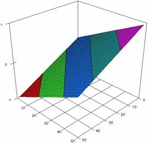
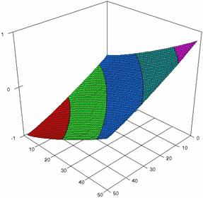
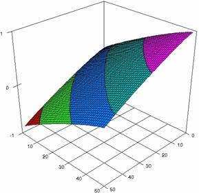
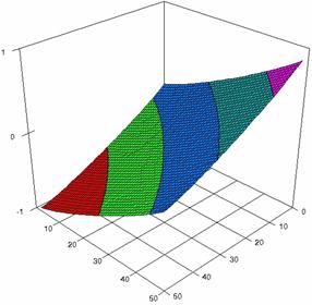
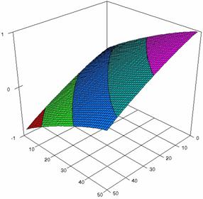
Figure 2. The representation of the ER values and its confidence limits obtained with DBinomialC and DAC methods at 0 < X, Y < m = n = 50
The upper and lower boundaries of confidence intervals obtained with DBinomial and DAC methods for equals sample sizes (m = n = 50) were represented graphical in figure 2, using a logarithmical scale. On horizontal axis were presented the values of the sample sizes (m = n) depending on binomial variables (X, Y) and on vertical axis the values of confidence intervals limits.
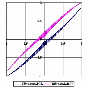
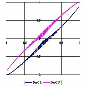
Figure 2. The upper and lower confidence interval limits (logarithmic scale)
for ER at 0 < X, Y < m = n = 50
The experimental errors for choused equal sample sizes (m = n) were imported in SlideWrite Plus program were the graphical representations were created (see figures 3 to 6). On X-axis were represented the values of X binomial variable, on Y-axis the values of Y binomial variable, and on Z-axis the values of the percentage of experimental errors for each specified methods. The graphical representations were created using a 3D-Mesh graph type with 80% perspective, 60° tilt angle and 75° rotation angle. Were represented with red color the experimental percentages from 0 to 2, with green the percentages from 2 to 4, with blue the percentages from 4 to 6, with cyan the percentages from 6 to 8, and with magenta the percentages from 8 to 10.
For equal samples sizes, the graphical representations of the percentages of the experimental errors calculated using specified methods were presented in figures 3 (m = n = 5), 4 (m = n = 10), 5 (m = n = 20), and 6 (m = n = 40).
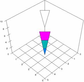
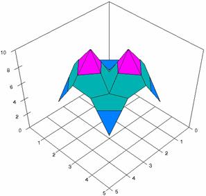
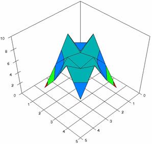
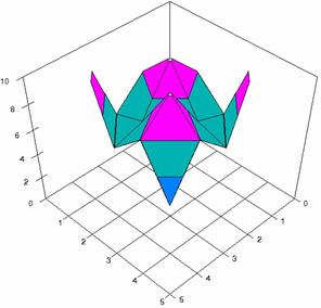
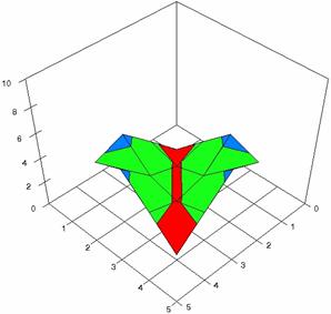
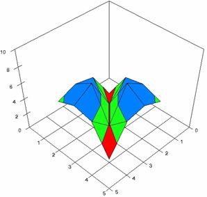
Figure 3. The ER percentages of the experimental errors with DWald, DAC, DAs, DAsC, DBinomial and DBinomialC at 0 < X, Y < m = n = 5
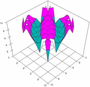
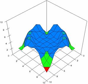
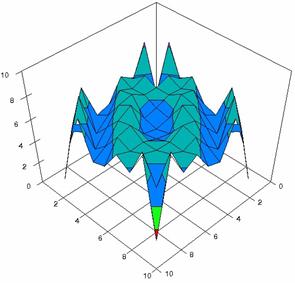
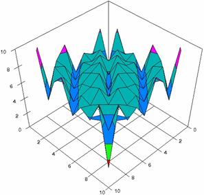
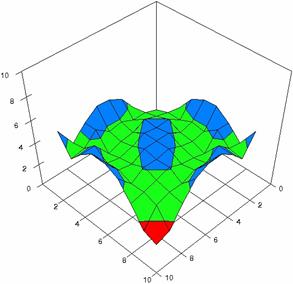
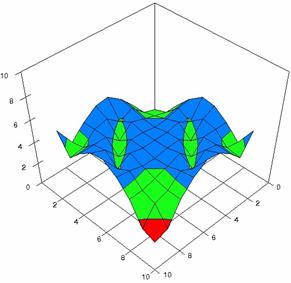
Figure 4. The ER percentages of the experimental errors with DWald, DAC, DAs, DAsC, DBinomial and DBinomialC at 0 < X, Y < m = n = 10
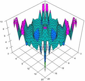
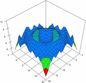
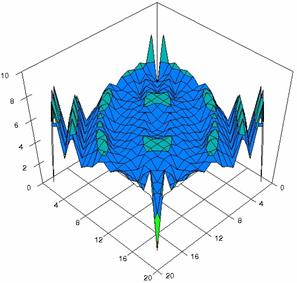
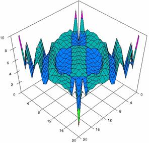
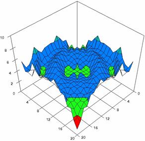
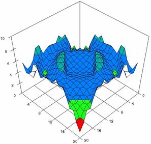
Figure 5. The ER percentages of the experimental errors with DWald, DAC, DAs, DAsC, DBinomial and DBinomialC at 0 < X, Y < m = n = 20
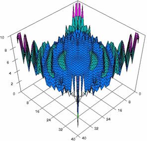
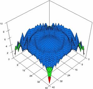
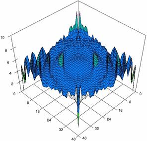
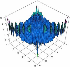
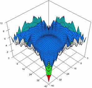
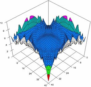
Figure 6. The percentages of the experimental errors obtained for excess risk with DWald, DAC, DAs, DAsC, DBinomial and DBinomialC at 0 < X, Y < m = n = 40
The averages (MErr) and standard deviations (StdDev) of experimental errors for equal sample sizes (m = n = 5, 10, 20, and 40) are in table 1.
|
m=n |
DWald |
DAC |
DAs |
DAsC |
DBinomial |
DBinomialC |
|
5 |
12.32 (4.13) |
6.53 (1.99) |
5.30 (2.30) |
7.65 (2.37) |
2.87 (1.36) |
3.70 (1.69) |
|
10 |
8.98 (2.80) |
4.44 (1.28) |
5.72 (1.62) |
6.60 (1.74) |
3.76 (0.97) |
3.99 (1.01) |
|
20 |
7.11 (2.01) |
4.90 (0.99) |
5.53 (0.96) |
6.14 (1.10) |
4.65 (0.93) |
4.97 (1.02) |
|
40 |
6.06 (1.22) |
4.88 (0.58) |
5.30 (0.58) |
5.62 (0.68) |
5.04 (0.88) |
5.29 (0.94) |
Table 1. The averages and standard deviations (into parenthesis) of experimental errors for excess risk at m = n = 5, 10, 20, 40
The assessment of the methods was carried on with a particular situation: X = Y and m = n = 4, 6,…204 (even number). The experimental data were imports in Microsoft Excel where the graphical representations were creates (figure 7). In the graphical representation, on horizontal axis were represented the m = n values depending on X = Y values and on the vertical axis the percentage of the experimental errors.
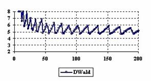
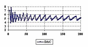
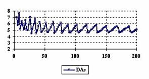
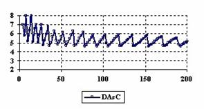
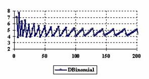
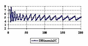
Figure 7. The experimental errors for excess risk ration at central point (X = Y) when
m = n = 4,6..200
The percentages averages (MErr) and the standard deviation (StdDev) of the experimental errors for central point estimation X = Y are in table 2.
|
Method |
DWald |
DAC |
DAs |
DAsC |
DBinomial |
DBinomialC |
|
MErr (Std Dev) |
5.67 (1.62) |
5.13 (0.60) |
5.29 (0.61) |
5.38 (0.71) |
4.73 (0.64) |
4.95 (0.61) |
Table 2. The MErr and StdDev for excess risk at X = Y when m = n = 4,6..204
The surface plots of dependences of the averages of the experimental errors (left side) and of the deviation relative to the significance level α = 5% (Dev5, right side) when sample sizes vary from 4 to 14 (m, n = 4..14) were graphically represented in figure 8.
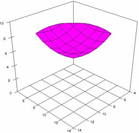
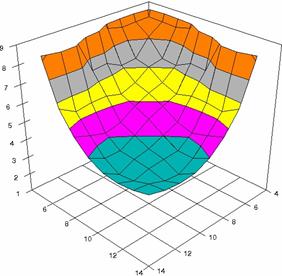
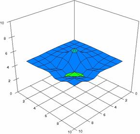
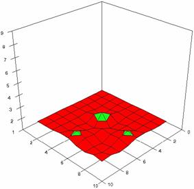
Figure 8. Dependences of the averages of experimental errors (left) and of deviation relative to the significance level α = 5% (right) for excess risk with DWald, and DAC
at m, n = 4..14
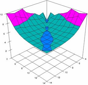
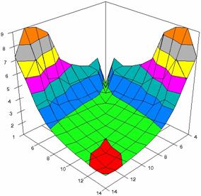
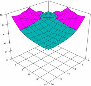
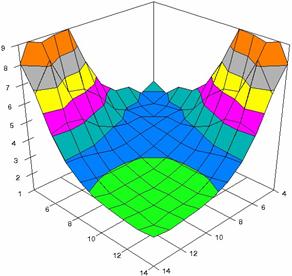
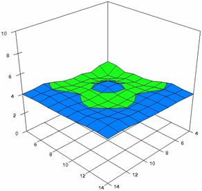
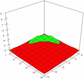
Figure 8. Dependences of the averages of experimental errors (left) and of deviations relative to the significance level α = 5% (right) for excess risk with DAs, DAsC, and DBinomial
at m, n = 4..14
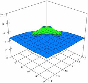
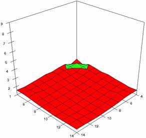
Figure 8. Dependences of the averages of experimental errors (left) and of deviations relative to the significance level α = 5% (right) for excess risk with DBinomialC at m, n = 4..14
The dependency surface plots were created with 80% perspective, 30° tilt angle and 45° rotation angle. For the graphical representation of the experimental errors average (left side graphics), with red color were represented the experimental values from 0 to 2, with green the values from 2 to 4, with blue the values from 4 to 6, with cyan the values from 6 to 8, and with magenta the values from 8 to 10. In the right side graphs, were represented with red color the experimental values from 1 to 2, with green from 2 to 3, with blue from 3 to 4, with cyan from 4 to 5, with magenta from 5 to 6, with yellow from 6 to 7, with gray from 7 to 8, and with rose from 8 to 9.
The averages of the averages of experimental errors (MMErr) and deviations relative to the imposed significance level (MDev5) for samples sizes which vary in 4..14 domain are in table 3:
|
Method |
DWald |
DAC |
DAs |
DAsC |
DBinomial |
DBinomialC |
|
MMErr (MDev5) |
12.20 (8.18) |
4.66 (1.62) |
7.07 (3.64) |
8.29 (4.28) |
3.87 (1.73) |
4.34 (1.59) |
Table 3. The MMErr and MDev5 scores for ER when samples sizes vary in 4..14 domain
Using the results obtained from the 100 random binomial variable (X, Y) and samples size (m, n) from 4 to 1000 domain, a set of calculations as are described in paper [7] are done and presented in tables 4-7 and represented in figure 9.
In the figure 9 were represented with black dots the frequencies of the experimental error for each specified method; with green line the best errors interpolation curve with a Gauss curve (dIG(er)). The Gauss curves of the average and standard deviation of the experimental errors (dMV(er)) were represented with red line, while the Gauss curve of the experimental errors deviations relative to the significance level (d5V(er)) with blue squares. The Gauss curves of the standard binomial distribution from the average of the errors equal with 100·α (pN(er,10)) were represented with black line.
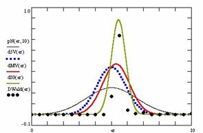
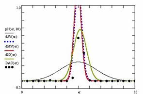
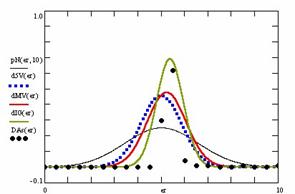

Figure 9. The pN(er, 10), d5V(er), dMV(er), dIG(er) and the frequencies of the experimental errors for each specified method and random X, m, Y, n (0 < X, Y < m, n; 4 ≤ m, n ≤ 1000)
Table 4 contains the average of the deviation of the experimental errors relative to significance level α =5% (Dev5), the absolute differences of the average of experimental errors relative to the imposed significance level (|5-M|), and standard deviations (StdDev).
|
No |
Method |
Dev5 |
Method |
|5-M| |
Method |
StdDev |
|
1 |
DAC |
0.32 |
DAC |
0.05 |
DAC |
0.32 |
|
2 |
DAs |
0.87 |
DAs |
0.23 |
DAs |
0.84 |
|
3 |
DAsC |
0.89 |
DAsC |
0.27 |
DAsC |
0.85 |
|
4 |
DWald |
0.90 |
DWald |
0.30 |
DWald |
0.85 |
Table 4. Methods ordered by performance according to Dev5, |5-M| and StdDev criterions
Table 5 contains the absolute differences of the averages that result from Gaussian interpolation curve to the imposed significance level (|5-MInt|), the deviations that result from Gaussian interpolation curve (DevInt), the correlation coefficient of interpolation (r2Int) and the Fisher point estimator (FInt).
|
No |
Method |
|5-MInt| |
Method |
DevInt |
Method |
r2Int |
FInt |
|
1 |
DAC |
0.17 |
DWald |
0.45 |
DAs |
0.77 |
64 |
|
2 |
DAs |
0.37 |
DAsC |
0.46 |
DAsC |
0.78 |
66 |
|
3 |
DWald |
0.45 |
DAs |
0.58 |
DWald |
0.78 |
68 |
|
4 |
DAsC |
0.45 |
DAC |
0.59 |
DAC |
0.79 |
71 |
Table 5. The methods ordered by |5-MInt|, DevInt, r2Int and FInt criterions
The superposition between the standard binomial distribution curve and interpolation curve (pNIG), the standard binomial distribution curve and the experimental error distribution curve (pNMV), and the standard binomial distribution curve and the error distribution curve around significance level (pN5V) are in table 6.
|
No |
Method |
pNIG |
Method |
pNMV |
Method |
pN5V |
|
1 |
DWald |
0.45 |
DAC |
0.35 |
DAC |
0.36 |
|
2 |
DAsC |
0.46 |
DAs |
0.69 |
DAs |
0.72 |
|
3 |
DAs |
0.54 |
DWald |
0.70 |
DAsC |
0.73 |
|
4 |
DAC |
0.55 |
DAsC |
0.70 |
DWald |
0.73 |
Table 6. Methods ordered by the pNIG, pNMV, and pN5V criterions
Table 7 contain the percentages of superposition between interpolation Gauss curve and the Gauss curve of error around experimental mean (pIGMV), between the interpolation Gauss curve and the Gauss curve of error around imposed mean (α = 5%) (pIG5V), and between the Gauss curve experimental error around experimental mean and the error Gauss curve around imposed mean α = 5% (pMV5V).
|
No |
Method |
pIGMV |
Method |
pIG5V |
Method |
pMV5V |
|
1 |
DAs |
0.81 |
DAs |
0.73 |
DAC |
0.94 |
|
2 |
DAsC |
0.71 |
DAC |
0.67 |
DAs |
0.89 |
|
3 |
DWald |
0.70 |
DAsC |
0.63 |
DAsC |
0.87 |
|
4 |
DAC |
0.67 |
DWald |
0.61 |
DWald |
0.73 |
Table 7. The confidence intervals ordered by the pIGMV, pIG5V, and pMV5V criterions
Discussions
Analyzing the graphical representation of the confidence boundaries (see figure 1 and 2) we could not said which method was better in excess risk confidence intervals estimation.
For equal sample sizes (m = n) the average of the experimental errors obtained with DWald method decrease with the increasing of the sample sizes. DAs and DAsC methods present for choused equal sample sizes averages of the experimental errors greater than 100·α. If we looked at the averages of the experimental errors obtained with DBinomial and DBinomialC methods we can observe that is increasing proportional with the increasing of the sample sizes. The DBinomialC method obtains systematically the lowest standard deviation.
Analyzing the results from the central point, X = Y, the lowest deviation relative to significance level 5% was obtains by the DAC (0.6) and DBinomialC (0.61) methods.
The closest average of the experimental errors to the imposed significance level (α = 5%) was obtains by the DBinomialC (4.95%) method followed by the DAC (5.13%) method. If we looked at the graphical representations (figure 7) it can be observed that the percentages of the experimental errors obtained with DWald method are greater than 8% when the values of the binomial variables (X, Y) are closed to 0 (2 ≤ X, Y ≤ 7).
Analyzing the results of the experiment conduct when the sample sizes vary 4 ≤ m, n ≤ 14 it can be observe that for three confidence interval methods (DWald, DAs, DAsC), the averages of experimental errors were greater than the expected value (α = 5%).
The DAC method was obtains the best estimation (an average of the errors equal with 4.66%). The lowest standard deviation was obtains by the DBinomiaC method closely followed by the DAC method.
If we look at the results of the random experiment (0 < X < m, 0 < Y < n, and 4 ≤ m, n ≤ 1000) we can be remarked that, the DAC method obtained the closest experimental error average to the significance levels α = 5% (table 4).
The lowest experimental standard deviation and the lowest deviation relative to the imposed significance level (α = 5%) was obtains also by the DAC method.
The DAC method also obtained the closed average of the interpolation errors to the significance level (α = 5%). The lowest interpolation standard deviation was obtains by the DWald method and the best correlation coefficient of interpolation was obtains by the DAC method.
The DAC method obtained the maximum superposition between the curve of interpolation and the curve of standard binomial distribution.
The DAsC, DWald and DWaldC methods obtained the maximum superposition between the curve of standard binomial distribution and the curve of experimental errors, and the maximum superposition between the curve of standard binomial distribution and the curve of experimental errors around the significance level (α = 5%).
The maximum superposition between the Gauss curve of interpolation and the Gauss curve of errors around experimental mean and the maximum superposition between the Gauss curve of interpolation and the Gauss curve of errors around significance level (α = 5%) was obtained by the DAs method.
The DAC method obtained the maximum superposition between the Gauss curve of experimental errors and the Gauss curve of errors distribution around imposed mean (α = 5%).
Conclusions
The DAC, DAs, DAsC, DBinomial, and DBinomialC methods of computing the confidence intervals for excess risk are superior compared with the asymptotic method (called here DWald).
For equal sample sizes (situation which is not common in research) the DAC method obtains the averages of the experimental errors more closed to the imposed values comparing with the other methods while the DBinomial method obtain the lowest standard deviation.
The DAC method become the method of computing confidence intervals for excess risk which obtain the best performances when the sample sizes vary from 4 to 14 and on random values for binomial variables (0 < X, Y < m, n) and random sample sizes (4 ≤ m, n ≤ 1000).
Based on these conclusions we recommend the DAC method for computing confidence intervals for excess risk instead of asymptotic method (DWald).
Acknowledgements
The first author is thankful for useful suggestions and all software implementation to Ph. D. Sci., M. Sc. Eng. Lorentz JÄNTSCHI from Technical University of Cluj-Napoca.
References