Binomial Distribution Sample Confidence Intervals Estimation
10. Relative Risk Reduction and RRR-like Expressions
Sorana BOLBOACĂ
“Iuliu Haţieganu” University of Medicine and Pharmacy, Cluj-Napoca, Romania
http://sorana.academicdirect.ro
Abstract
In trial, when the results are reported as dichotomies variables, the most important measure of effect are represented by the relative risk reduction, absolute risk reduction and number needed to treat, providing the basis for clinicians to balance the benefits and harms of therapy for their patients. The relative risk reduction is a very useful parameter in assessment of a treatment effect if it is accompanied by confidence intervals. The only method used in medical article for computing the confidence intervals for relative risk reduction is the asymptotic method. The aim the research was to propose some new methods of computing confidence intervals for relative risk reduction and relative risk reduction like parameters and to compare these methods with the asymptotic one in order to assess their performance.
In order to estimate the confidence intervals for relative risk reduction we proposed based on the literature definitions and on our experiences in confidence intervals five methods called here ARPWald, ARPAC, ARPWaldC1, ARPWaldC2, and ARPWaldC3. The criterions of assessment were represented by the upper and lower boundaries, the average of experimental errors and standard deviations, and the deviation relative to imposed significance level α equal with 5%. All methods were assessed on random variables (X, Y) and random samples sizes (n, m).
Chousing a method of computing confidence intervals for relative risk reduction (RRR) and RRR-like functions depend on objective of research. If we desire a method which to obtain performance in estimating the average of the experimental errors we can chouse the ARPWald method, while if we need a method with the smallest deviation we will chouse the ARPAC method.
Keywords
Confidence Intervals Estimation; Relative Risk Reduction; Relative Risk Increase; Relative Benefit Increase
Introduction
Physicians are influenced of the modality of presenting the results of a therapy study because depending on which measures of effect choused, the impact of an intervention may appear large or small, even though the underlying data are the same [[1]]. The most important measure of effect are represented by the relative risk reduction, absolute risk reduction and number needed to treat [[2]]. When available, trial results regarding relative risk reductions (or increases), combined with estimates of baseline (untreated) risk in individual patients, provide the basis for clinicians to balance the benefits and harms of therapy for their patients [1, 2].
When the experimental treatment reduces the probability of a bad outcome the relative risk reduction can be computed. The relative risk reduction is defined as ״the proportional reduction in rates of bad outcomes between experimental and control participants in a trial״ [1, [3]] and is a very useful parameter in assessment of a treatment if it is accompanied by a confidence intervals. When the experimental treatment increases the probability of a good outcome, based on the same mathematical formula, the relative benefit increase (the proportional increase in rates of good outcomes between experimental and control patients in a trial) can be computed. The relative risk increase (the proportional increase in rates of bad outcomes between experimental and control patients in a trial) can be computed based on the same formula when the experimental treatment increase the probability of a bad outcome.
The confidence limits for the relative risk reduction are 1 minus the confidence limits for the relative risk [[4], [5], [6]]. Unfortunately, the only method reported in medical literature for relative risk increase is the asymptotic method that is well known that provide too short confidence intervals [4, 5].
The aim of this paper was to propose some new methods of computing confidence intervals for relative risk reduction and relative risk reduction like parameters and to compare these methods with the asymptotic one in order to assess their performance.
Materials and Methods
Mathematically, the relative risk reduction is equals with 1 minus relative risk (1-Xn/(Ym)), noted with ci9 in the program [[7]].
In order to estimate the confidence intervals for relative risk reduction were proposed based on the literature definitions and on the experience in confidence intervals estimation [7, [8]], five functions:
![]() (1)
(1)
![]() (2)
(2)
![]() (3)
(3)
![]() (4)
(4)
![]() (5)
(5)
The functions described above were implemented into a PHP program that allowed estimating their performance. The PHP functions were:
function ARPAC($X,$m,$Y,$n,$z,$a){ return ARP("RPAC",$X,$m,$Y,$n,$z,$a);}
function ARPWald($X,$m,$Y,$n,$z,$a){ return ARP("RPWald",$X,$m,$Y,$n,$z,$a);}
function WaldC1($X,$m,$Y,$n,$z,$a){
if($Y){ $P = $X*$n/$Y/$m;
if($X){ $t = ($m-$X)/($X+pow(($m/$X+$X/$m)/$m,0.25))/$m + ($n-$Y)/
($Y+pow(($n/$Y+$Y/$n)/$n,0.25))/$n;
return array ( $P * exp(-$z * sqrt($t)) , $P * exp($z * sqrt($t)));
} else return array ( 0, $n * pow($a/2,1/$m)/$Y );
}else{ return array ( $X/$m/pow($a/2,1/$n) , (float)"INF" ); }}
function ARPWaldC1($X,$m,$Y,$n,$z,$a){ return ARP("WaldC1",$X,$m,$Y,$n,$z,$a);}
function WaldC2($X,$m,$Y,$n,$z,$a){
if($Y){ $P = $X*$n/$Y/$m;
if($X){
$t = ($m-$X)/($X+pow(1-$X/$Y/$m,1/$n))/$m + ($n-$Y)/($Y+pow(1-$Y/$X/$n,1/$m))/$n;
return array ( $P * exp(-$z * sqrt($t)) , $P * exp($z * sqrt($t)));
} else return array ( 0, $n * pow($a/2,1/$m)/$Y );
}else{ return array ( $X/$m/pow($a/2,1/$n) , (float)"INF" ); }}
function ARPWaldC2($X,$m,$Y,$n,$z,$a){ return ARP("WaldC2",$X,$m,$Y,$n,$z,$a);}
function WaldC3($X,$m,$Y,$n,$z,$a){
if($Y){ $P = $X*$n/$Y/$m;
if($X){
$t = ($m-$X)/($X+pow(1-$X/$Y/$m,1/$m))/$m + ($n-$Y)/($Y+pow(1-$Y/$X/$n,1/$n))/$n;
return array ( $P * exp(-$z * sqrt($t)) , $P * exp($z * sqrt($t)));
} else return array ( 0, $n * pow($a/2,1/$m)/$Y );
}else{ return array ( $X/$m/pow($a/2,1/$n) , (float)"INF" ); }}
function ARPWaldC3($X,$m,$Y,$n,$z,$a){ return ARP("WaldC3",$X,$m,$Y,$n,$z,$a);}
The methods were assessed using as criterions the means of experimental errors (ErrM), the standard deviation of the experimental errors (called StdDev), and the deviation relative to imposed significance level α = 5% (called Dev5). The standard deviation was given by the formula:
 (6)
(6)
where n is the sample size.
The formula for deviation relative to the imposed significance level (α = 5%) was:
 (7)
(7)
The experiments were run for a 100∙(1-α) = 95% confidence interval, and a significance level of α = 5%, parameter noted with a in our PHP modules (sequence define("z",1.96); define("a",0.05); in the program, see [7]).
The program run uses the following execution line to compute for all methods a specified task:
$c_i=array("ARPWald", "ARPAC", " ARPWaldC1", " ARPWaldC2", " ARPWaldC3");
First, were computed and graphical represented the upper and lower boundaries for two implemented methods (ARPWald, ARPWaldC1) and for equal sample sizes (m = n = 50):
define("N_min",50); define("N_max",51); est_ci2_er(z,a,$c_i,"ci9","ci");
In order to choose some best confidence intervals for the relative risk reduction (ci9 function; f(X,m,Y,n) = 1-Xn/(Ym)), were analyzed the means of experimental errors and the associated standard deviation. For this experiment were choosing the next samples size 10, 20, and 50. The sequences of the program which allowed us to perform this experiment were:
· For m = n = 10:
define("N_min",10); define("N_max",11); est_ci2_er(z,a,$c_i,"ci9","er");
· For m = n = 20 was modified:
define("N_min",20); define("N_max",21);
· For m = n = 50 was modified:
define("N_min",50); define("N_max",51);
The assessment of the confidence intervals was carried on with a particular situation: m=n= 2,4..204 (m, n even number) and X = Y. The sequence of the program was:
define("N_min", 2); define("N_max",205); est_C2(z,a,$c_i,"ci9");
The dependences of the deviation average relative to the significance level (α = 5%) when sample sizes vary from 4 to 24 (4 < m, n < 25) and central point (X = Y) were computed using the next sequence of the program:
define("N_min", 4); define("N_max",25); est_C2(z,a,$c_i,"ci9", "ra");
In order to compare the errors of confidence intervals for the relative risk reduction, the experimental errors and standard deviations for all methods (ARPWald, ARPWaldC1, ARPWaldC2, ARPWaldC3, ARPAC) and 100 random X, Y and random m, n ( 4 ≤ X, Y < m, n ≤ 1000). The sequence of the program was:
define("N_min", 4); define("N_max",1000); est_ci2_er(z,a,$c_i,"ci9","ra");
Results
The upper and lower confidence boundaries for relative risk reduction at m = n = 50 were obtained and were graphically represented (see figure 1 and 2) using the asymptotic method (ARPWald) and an adjusted asymptotic method (ARPWaldC1).
The 3D representations of lower and upper boundaries are in figure 1, using the SlideWrite Plus program. The Slide representations (figure 1) were created using a 3D-Mesh graph type with 80% perspective, 45° tilt angle and 30° rotation angle. On X-axis are represented the X values, on the Y-axis the Y values and on the Z the lower or upper confidence interval boundaries for the confidence intervals estimation. There are represented with red color the experimental values from 0 to 1, with green the values from 1 to 2, with blue the values from 2 to 3, with cyan the values from 3 to 4, and with magenta the values from 4 to 5.
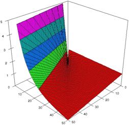
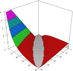
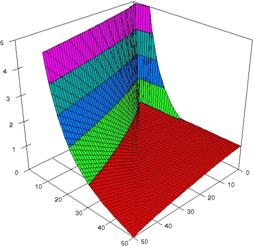
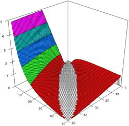

Figure 1. The representation of the relative risk reduction and its confidence boundaries obtained with ARPWald, and ARPWaldC1 at 0 < X, Y < m = n = 50
The upper and lower confidence boundaries were graphical represented using Microsoft Excel where on horizontal axis were represented the m = n values depending on X = Y values and on vertical axis the values of confidence boundaries (figure 2).
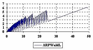
Figure 2. The upper and lower confidence boundaries for relative risk reduction with ARPWald and ARPWaldC1 at 0 < X, Y < m = n = 50
For choused samples sizes, using the SlideWrite Plus program, the 3D-graphical representation are performed based on the experimental data. For m = n = 10 the experimental error were presented in figure 3; for m = n = 20 in figure 4 and for m = n = 50 in figure 5. The graphics are created using the characteristics described above.
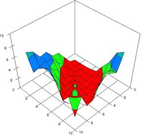
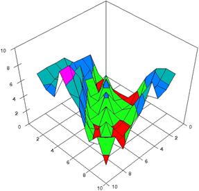
Figure 3. The experimental errors for RRR with ARPWald, ARPWaldC1 at 0<X, Y<m=n=10

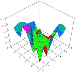
Figure 3. The experimental errors for RRR with ARPWaldC2, ARPWaldC3 at 0<X,Y<m=n=10
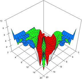
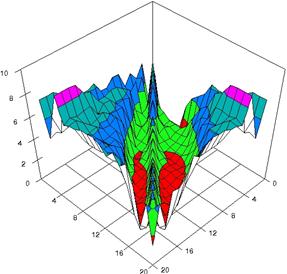
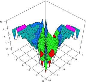

Figure 4. The experimental errors for RRR with ARPWald, ARPWaldC1, ARPWaldC2, and ARPWaldC3 at 0 < X, Y < m = n = 20
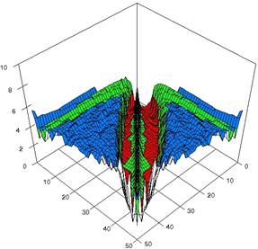
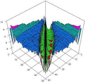
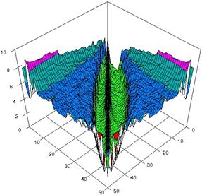

Figure 5. The experimental errors for relative risk reduction obtained with ARPWald, ARPWaldC1, ARPWaldC2, and ARPWaldC3 at 0 < X, Y < m = n = 50
The average of experimental errors (ErrM) and standard deviations (StdDev) for all method are presented in table 1.
Table 1. The average of experimental errors and standard deviations (parentheses) in
confidence interval estimation for relative risk reduction at m = n = 10, 20, and 50
|
Method |
ARPWald |
ARPWaldC1 |
ARPWaldC2 |
ARPWaldC3 |
|
10 |
2.25 (2.10) |
3.87 (2.41) |
4.11 (2.55) |
4.11 (2.55) |
|
20 |
2.90 (1.75) |
4.30 (2.14) |
4.64 (2.20) |
4.64 (2.20) |
|
50 |
3.64 (1.32) |
4.51 (1.61) |
4.83 (1.69) |
4.83 (1.69) |
The experiment at the central point was performed and the results were (table 2) imported in Microsoft Excel where the graphical representations are created (figure 6). In the graphical representation, on horizontal axis are represented the m = n values depending on X = Y values and on the vertical axis the percentages of the experimental errors.
Table 2. The average of the experimental error (ErrM) and standard deviations (StdDev) for
relative risk reduction at central point (X=Y) and m = n = 4,6..200
|
Method |
ARPWald |
ARPWaldC1 |
ARPWaldC2 |
ARPWaldC3 |
ARPAC |
|
ErrM |
4.51 |
4.99 |
5.11 |
5.11 |
4.40 |
|
StdDev |
0.76 |
0.69 |
0.66 |
0.66 |
1.04 |
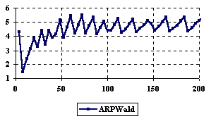
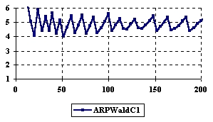
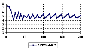
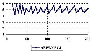
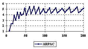
Figure 6. The variation of the experimental errors for relative risk reduction at central point
X = Y and m = n = 4,6..200
The three dimensional representation of the average of standard deviation reported to the imposed value (α = 5%) for relative risk reduction obtained with ARPWald, ARPWaldC1, ARPWaldC2 and ARPWaldC3 at 4 < m, n < 25 and X = Y are presented in figure 7. In the surface plot, there were represented with red color the experimental values between 0 - 1%, with green color the experimental values between 1 and 2%, with blue the values between 2 and 3%, with cyan the values between 3 and 4%, and with magenta the values between 4 and 5%. The graphics were created in Slide program with 80% perspective, 45° tilt angle and 15° rotation angle.
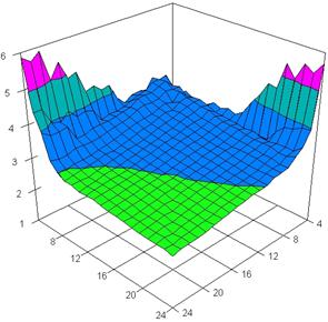
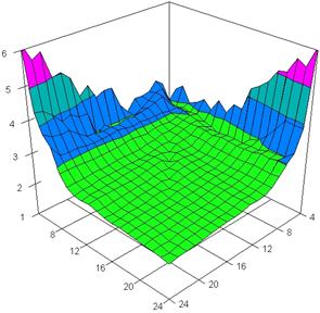
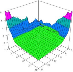
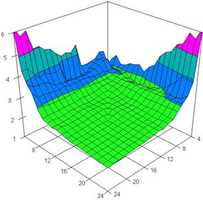
Figure 7. Dependences of the standard deviation relative to α = 5% for relative risk reduction with ARPWald, ARPWaldC1, ARPWaldC2, and ARPWaldC3 at X = Y and 4 < m, n < 25
Based on the results obtained from the random variables (X, Y) and random samples sizes (m, n), the frequencies of the experimental error (black dots) for each specified method, the best errors interpolation curve with a Gauss curve (dIG(er), green line), the Gauss curves of the average and standard deviation of the experimental errors (dMV(er), red line), the Gauss curve of the experimental errors deviations relative to the significance level (d5V(er), blue squares), and the Gauss curve of the standard binomial distribution relative to an average of the experimental errors equal with 100·α (pN(er,10), black line) are presented in figure 8.
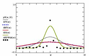
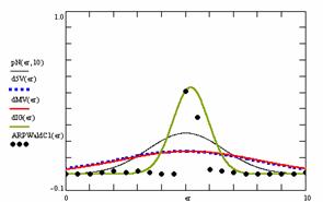

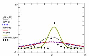
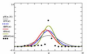
Figure 8. The pN(er, 10), d5V(er), dMV(er), dIG(er) and the frequencies of the experimental errors for random variables and sample sizes (1 ≤ X,Y < 1000, 4 ≤ m, n ≤ 1000)
For the random samples (m, n) and random binomial variables (X, Y), the results were presented in tables 3 to 6.
In table 3 were presented of the standard deviation of the experimental errors relative to significance level α =5% (Dev5), the average of the experimental errors relative to the significance level (|5-M|), and the average of the standard deviation of the experimental errors (StdDev).
Table 3. Methods ordered by performance according to Dev5, |5-M| and StdDev criterions
|
Nr |
Method |
Dev5 |
Method |
|5-M| |
Method |
StdDev |
|
1 |
ARPAC |
1.10 |
ARPWald |
0.11 |
ARPAC |
1.05 |
|
2 |
ARPWaldC1 |
2.88 |
ARPWaldC1 |
0.15 |
ARPWaldC2 |
2.88 |
|
3 |
ARPWaldC2 |
2.90 |
ARPWaldC2 |
0.32 |
ARPWaldC3 |
2.88 |
|
4 |
ARPWaldC3 |
2.90 |
ARPWaldC3 |
0.32 |
ARPWaldC1 |
2.88 |
|
5 |
ARPWald |
2.92 |
ARPAC |
0.32 |
ARPWald |
2.92 |
The table 4 presented the average of the interpolated errors relative to significance level (|5-MInt|), the standard deviation of interpolation (DevInt), the correlation between interpolation curve and experimental results and the Fisher point estimator.
Table 4. The methods ordered by |5-MInt|, DevInt, r2Int and FInt criterions
|
Nr |
Method |
|5-MInt| |
Method |
DevInt |
Method |
r2Int |
FInt |
|
1 |
ARPWald |
0.05 |
ARPWaldC1 |
0.75 |
ARPWald |
0.65 |
35 |
|
2 |
ARPAC |
0.06 |
ARPWald |
0.81 |
ARPAC |
0.65 |
36 |
|
3 |
ARPWaldC1 |
0.22 |
ARPAC |
0.84 |
ARPWaldC2 |
0.68 |
40 |
|
4 |
ARPWaldC2 |
0.44 |
ARPWaldC2 |
0.85 |
ARPWaldC3 |
0.68 |
40 |
|
5 |
ARPWaldC3 |
0.44 |
ARPWaldC3 |
0.85 |
ARPWaldC1 |
0.71 |
48 |
The superposition between the standard binomial distribution curve and interpolation curve (pNIG), the standard binomial distribution curve and the experimental error distribution curve (pNMV), and the standard binomial distribution curve and the error distribution curve around significance level (pN5V) were presented in table 5.
Table 5. Methods ordered by the pNING, pNMV, and pN5V criterions
|
Nr |
Method |
pNIG |
Method |
pNMV |
Method |
pN5V |
|
1 |
ARPWaldC1 |
0.65 |
ARPWald |
0.71 |
ARPWald |
0.71 |
|
2 |
ARPWaldC2 |
0.69 |
ARPWaldC2 |
0.71 |
ARPWaldC2 |
0.71 |
|
3 |
ARPWaldC3 |
0.69 |
ARPWaldC3 |
0.71 |
ARPWaldC3 |
0.71 |
|
4 |
ARPAC |
0.70 |
ARPWaldC1 |
0.72 |
ARPWaldC1 |
0.72 |
|
5 |
ARPWald |
0.99 |
ARPAC |
0.79 |
ARPAC |
0.83 |
Table 6. The confidence intervals ordered by the pIGMV, pIG5V, and pMV5V criterions
|
Nr |
Method |
pIGMV |
Method |
pIG5V |
Method |
pMV5V |
|
1 |
ARPAC |
0.82 |
ARPAC |
0.87 |
ARPWald |
0.90 |
|
2 |
ARPWaldC2 |
0.47 |
ARPWaldC2 |
0.47 |
ARPWaldC1 |
0.90 |
|
3 |
ARPWaldC3 |
0.47 |
ARPWaldC3 |
0.47 |
ARPWaldC2 |
0.88 |
|
4 |
ARPWald |
0.45 |
ARPWald |
0.45 |
ARPWaldC3 |
0.88 |
|
5 |
ARPWaldC1 |
0.43 |
ARPWaldC1 |
0.43 |
ARPAC |
0.88 |
In the table 6 are the percentages of superposition between interpolation Gauss curve and the Gauss curve of error around experimental mean (pIGMV), between the interpolation Gauss curve and the Gauss curve of error around imposed mean (α = 5%) (pIG5V), and between the Gauss curve experimental error around experimental mean and the error Gauss curve around imposed mean α = 5% (pMV5V).
Discussions
Two-dimensional representation of the upper and lower confidence boundaries (figure 2) was more useful in comparing the implemented methods comparing with three-dimensional representations (figure 3), because even if there were differences between estimated boundaries these differences could not be saw on 3D-representations.
Analyzing the experimental data obtained in assessment of confidence interval for relative risk reduction we can observed that for m = n = 10, 20, and 50 the best performance were obtained with ARPWaldC2 and ARPWaldC3 methods if we looked at the experimental errors average. If we need a confidence interval with the lowest standard deviation, we can say that the ARPWald method is the method which can be used. As we can saw, the average of the experimental errors for relative risk reduction were always less then the imposed value (α = 5%) and increase with increasing of the sample size but never exceed 5% until m = n = 50.
If we look at the estimation for the central point (X = Y), when m = n vary in from 4 to 200 (m = n = even number) ARPWaldC1 method obtained systematically performance, presenting the average of the experimental error more closed to the imposed value (α = 5%) compared with the other methods; the ARPWaldC1 method was followed by the ARPWaldC2 and ARPWaldC3 methods.
Analyzing the performance of the implemented methods on random variables and random samples sizes we can observed that the ARPWald method obtained the average of the experimental error more closed to the imposed values (α = 5%) comparing with other methods. The ARPAC method obtained the lowest experimental standard deviation and the most closed experimental standard deviation to the imposed value (α = 5%). Again the ARPWald method obtained the errors average of interpolation more closed to the imposed value (α = 5%) while the ARPWaldC1 method obtained the lowest interpolation standard deviation and the best correlation between theoretical curve and experimental data (table 4). The ARPWald method obtained the maximum superposition between the curve of interpolation and the curve of standard binomial distribution. The maximum superposition between the curve of standard binomial distribution and the curve of errors distribution around the imposed value (α = 5%), and the maximum superposition between the curve of standard binomial distribution and the curve of experimental errors distribution was obtained by the ARPAC method. The maximum superposition between the Gauss curve of interpolation and the Gauss curve of errors around experimental mean and the maximum superposition between the Gauss curve of interpolation and the Gauss curve of errors around imposed value (α = 5%) was obtained by the ARPAC method (table 6). The ARPWald obtained the maximum superposition between the Gauss curve of experimental errors and the Gauss curve of errors around imposed mean (α = 5%).
Conclusions
Chousing a method of computing the confidence intervals for relative risk reduction and relative risk reduction like functions depend on the objectives of the researcher. If we wand a methods which to obtained am average of the experimental errors more closed to the imposed significance level (5% for example) the ARPAC or ARPWald methods can be choused. If we wish to obtain the lowest standard deviation, which means the lowest variation between experimental results the ARPAC method can be chouse.
Even if the mathematical formulas of the ARPWaldC2 and ARPWaldC3 methods were different, there was no significance differences between the in estimating the confidence interval for relative risk reduction between these two methods.
Acknowledgement
The author is thankful for useful suggestions and all software implementation to Ph. D. Sci., M. Sc. Eng. Lorentz JÄNTSCHI from Technical University of Cluj-Napoca.
References