The Analysis of the Two-dimensional Diffusion Equation

With a Source

Victor Onomza WAZIRI^1*, Sunday Augustus REJU²

^1*Mathematics/Computer Science Department, Federal University of Technology, Minna 920003, Niger State, Nigeria; ^*corresponding author; ²National Open University of Nigeria, Victoria Island, Lagos, Nigeria

dronomzawaziri@yahoo.com, sreju@nou.edu.ng

Abstract

This study presents a new variant analysis and simulations of the two-dimensional energized wave equation remarkably different from the diffusion equations studied earlier studied. The objective functional and the dynamical energized wave are penalized to form a function called the Hamiltonian function. From this function, we obtained the necessary conditions for the optimal solutions using the maximum principle. By applying the Fourier solution to the first order differential equation, the analytical solutions for the state and control are obtained. The solutions are simulated to give visual physical interpretation of the waves and the numerical values.

Keywords

Maximum principle, Hamiltonian function, Fourier series, energized wave equation and Simulates

Introduction

Consider an optimization problem:

                                                1

subject to the dynamical constraint energized wave equation:

                                   2

The unconstrained equation is formulated by augmenting equations 1 and 2 by penalizing the equations using the penalty function μ(x, y, t) ≥ 0 (function to be determined in (Waziri and Reju, 7):

3

The Hamiltonian function

The unconstrained formulation of equations 1 and 2 is achieved by penalizing the constrained equation to obtain the Hamiltonian function as in (Singh et al, 4). The Hamiltonian function is defined:

            4

where  is continuous penalty function

The maximum principle

The first order necessary conditions for optimality; also known as the maximum principle to the Hamiltonian function 4 is equivalently expressed as:

                                                            5

We note by definition akin to (Singh et al. ibid), the derivative with respect to the penalty λ:

                                                                                            6

also by definition:

                                                                                                                      7

                                                                                                        8

implying that:

                                                                                                          9

Differentiating equation 7 with respect to t-variable yields:

                                                                                                                 10

Equating equations 6 and 10 result in a first order partial differential equation:

                                                                                                 11

Equation 11 shows that the rate of change of optimal control is the optimal state.

Suppose that equation 11 has a Fourier series solution as proposed by (Duchateau et al., 1), then:

                                                                                12

                                                                               13

But from equation 11, we must have that:

                                                                                    14

Comparing the α_i with the u_it in equations 14 and 13 show that α_i = u_it.

Fourier series representation of the energized wave problem

This section formulates the two-dimensional energized wave equation problem in consonance with the Fourier series solutions. We note that the following under numerates as derived from section 1 above are without contradictions:

                                                                           15

                                                                              16

                                                              17

                                                              18

                                                                                19

Substituting all the derived Fourier solutions 15 through to 19 into the dynamical constraint equation 2, yields:

     20

Equation 20 is comparably equivalent to equation 2. Hence factorizing 20, yields the third order differential system:

                                                                                21

Therefore an equivalent representation to the constraint equation is:

                                                                                            22

The quadratic objective functional 1 has equivalence in Fourier series solution    and is here given in vector integral form:

                     23

Thus in view of equations 12 and 13, the optimization problem has         equivalence in vector integral formulations:

                     24

subject to the dynamical constraint equation:

                                                                                        25

Comparing equations 3 , 24, the unconstrained equivalence is defined:

                                         26

Let us reconsider the general equation 25. The nth third order partial differential equation is given by:

                                                                                     27

The characteristic to equation 27 is written simply:

                                                                                             28

Solving the characteristic equation

The roots of the characteristic equation 28 are:

                                     29

                   30

                             31

The roots are a real and a pair of conjugates complex roots. By De-Moivre’s theorem, we transform the conjugate roots into a set of real equivalence roots. By the choice of one equivalence real root, we have two real roots.  Thus suppressing the variables x and y, we have:

                                                                                   32

With t=0, equation 32 becomes:

                                                                     33

implying that:

                                                                                    34

Taking the partial derivative of equation 32 with respect to t-variable yields:

                                                                               35

Once more by setting t=0 in equation 35, we obtain:

                                                               36

From equation (34), equation 36 yields:

                       37

Putting equation 37 in to 34, yields:

                           38

From equations 37 and 38, it is not difficult to see that equation 32 becomes:

            39

But u(0,0,t) = u(1,y,t) = u(x,1,t) = u(1,1,t) = 0 by definition. Therefore, we deduce that ; whence . With this final deduction, we have:

                                    40

Furthermore, since the rate of change of the optimal control is the state, then:

                                    41

Equations 40 and 41 are our desired analytical optimal control and state respectively.

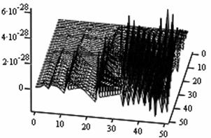
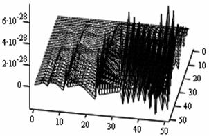
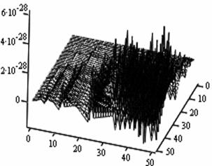
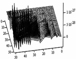
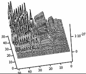
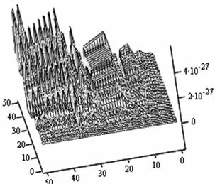
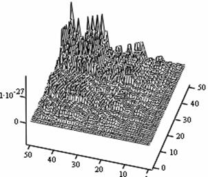
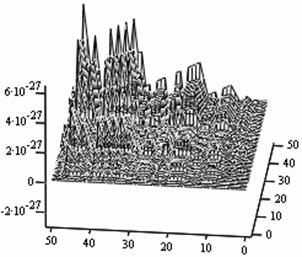
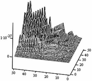
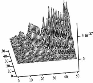
The simulation of the analytical optimal solutions of equation

The following figures below correspond to different simulates obtained under various dimensional spaces (Figure 1-18). The meshes and the argument iterate remain constant.

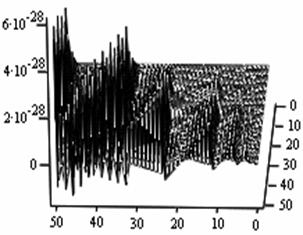
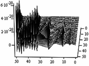
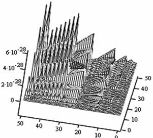
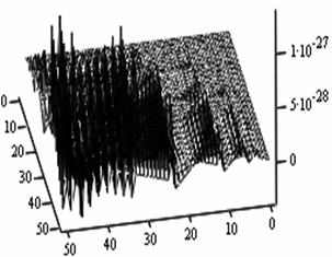
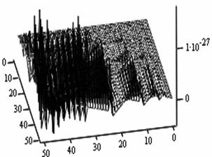
Figure 1. The control simulate at n = 2	Figure 2. The state simulate at n = 2

Figure 3. The control simulate at n = 5	Figure 4. The state simulate at n = 5

Figure 5. The control simulate at n = 10	Figure 6. The state simulate at n = 10

Figure 7. The control simulate at n = 20	Figure 8. The state simulate at n = 20

Figure 9. The control simulate at n = 30	Figure 10. The state simulate at n = 30

Figure 11. The control simulate at n = 35	Figure 12. The state simulate at n = 35

Figure 13. The control simulate at n = 40	Figure 14. The state simulate at n = 40

Figure 15. The control simulate at n = 50	Figure 16. The state simulate at n = 50

Figure 17. The control simulate at n = 60	Figure 18. The state simulate at n = 60

Analysis of Simulated Outputs

The table below (table 1) gives us the general numerical simulated values for the problem (P1).

If we take the upper most numerical values as our numerical solutions from each of the Simulates, table 1 summaries the outputs.

Table 1. Simulated outputs optimal values

s/n	Dimensional space n	Control u(x,y,t)	Control z(x,y,t)
1	2	6 · 10^-28	6 · 10^-28
2	5	6 · 10^-28	1 · 10^-27
3	10	6 · 10^-28	1 · 10^-27
4	20	6 · 10^-27	1 · 10^-27
5	30	1 · 10^-27	4 · 10^-27
6	40	6 · 10^-28	2 · 10^-27
7	50	1 · 10^-27	5 · 10^-27
8	60	1 · 10^-27	5 · 10^-27

General comments on the simulates and the outputs values

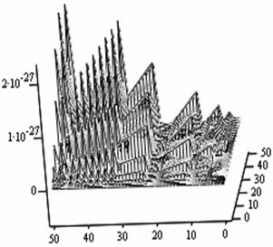
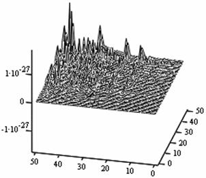
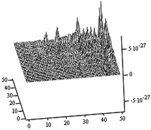
1. A cursory observation of table 1 shows the control and the states at different strata maintain stability. This clearly portrays the fact that the controls and state trajectories converge.

2. The analytical optimal States and controls are dominantly boundary solutions;           while some portions of the controls and States are partially stable with some blocky waves scattered far below the more conspicuous disturbed edge boundaries.

3. The Simulates reveal more energized waves propagation; especially at the regimes near the edges of the Simulates when the n profiles are at planes 30, 35, 40 and 60.

4. While other edges of the Simulates exhibit conspicuous higher disturbances, the other extreme ends are remarkably at lower states of agitations. Thus it takes more controlling energy to stabilize the controls and states at the disturbed boundaries than at the other relatively undisturbed edges.

5. Some Simulates resembles some subduction zones with better analytical depth characterizing some known tectonic dynamical processes. These phenomena exhibit the physical prominent aftermath of distortions when the strata are at the space levels 30 and 60.

6. Table 1 shows that the optimized values progressively become larger as the             sizes of the spatial planes are increased.

7. In view of the numerical values demonstrated, one may conclude that the control and state characterize relatively insignificant values. In other words, the wave’s wavelengths are of short magnitudes construing some high packages of energy.

Conclusions

We have obtained the analytical optimal solutions of the two-dimensional energized wave equation using the Hamiltonian forms. The Simulates give us visual interpretation of the optimized solutions.

The analytical solutions would enhance further computational processes using the ECGM algorithm towards the derivation of the optimal controls for states and controls at various spatial planes.

References

[1]     Duchateau P., Zachmann D. W., Partial differential equations. Mcgraw-Hill publishing, 1986.

[2]     Ibiejugba M. A., Onumanyi P., On control operator and some of its applications. J. Math. Analy. Applic., 103, 1984, p. 31-7.

[3]     Reju S. A. Computational Optimization in Mathematical physics, Ph.D. Thesis, Univ. of Ilorin, Ilorin, Nigeria, 1995.

[4]     Singh M. A., Titli A. J., System Decomposition, Optimizatio and Control; Pergamon, Tou Louse  France, 1978.

[5]     Waziri V. O., Optimal Control of Energized Wave equations using the Extended Conjugate Gradient Method (ECGM). Ph.D. Thesis, Federal Univ. of Technology, Minna, Nigeria, 2004.

[6]     Waziri V. O., Reju S. A., Control Operator for the Two-Dimensional Energized Wave Equation. Control Operator for the Two-Dimensional Energized Wave Equation, Leonardo Journal of Science, Romania, ISSN 1583-0233, Issue 9, July-December, 2006, p. 33-44.