Conjugate Gradient Method with Ritz Method for the Solution of Boundary Value Problems

Victor Onomza WAZIRI and Kayode Rufus ADEBOYE

Mathematics/ Computer Science Department, Federal University of Technology, Nigeria

dronomzawaziri@yahoo.com, professorkradeboye@yahoo.com

Abstract

In this paper, we wish to determine the optimal control of a one-variable boundary value problem using the Ritz algorithm. The posed optimal control problem was inadequate to achieve our goal using the Conjugate Gradient Method version developed by (Harsdoff, 1976). It is anticipated that other operators from some given different problems may sustain the application of the algorithm if the approximate solutions terms are properly chosen quadratic functionals. The graphical solution given at the end of section five of the paper, however, shows that our problem can not have an optimal minimum value since the minimum output is not unique. The optimal value obtained using Mathcad program codes may constitute a conjugate gradient approximate numerical value. As observed from the graphical output, Ritz algorithm could give credence for wider horizon in the engineering computational methods for vibrations of mechanical components and simulates.

Keywords

Conjugate gradient method (CGM), extended conjugate gradient method (ECGM), optimal control, boundary values problem (BVP), Ritz algorithm, variational method.

Introduction

The Ritz method is a variational method. Variational methods are approximate methods for the solutions of boundary value problems (BVP). These methods include the Collocation, Garlerkin (with its various versions; Adeboye (1997)), least squares methods and the moment methods; amongst others. In each variational algorithm, we obtain some coefficients of some given assumed approximate solutions to the BVP that would satisfy some boundary given conditions.

In this piece of work, we wish to verify whether the Ritz method solution for a given BVP can be posed as a further step for obtaining optimal control variables This is sequel to the acquisition of the approximate solutions of a well-posed BVP containing a two-term approximate solution functional.

Theory of the Ritz Method

Many versions of Ritz method abound; as can be inferred from (Gilbert et al, 1973) and (Richard et al, 1988). In this study, we consider the version credited to (Jain, 1984): Jain considers a functional:

(2.1)

Assume a function u(x) derived from (2.1) for which the integral J[u] takes on a maximum or minimum value and which satisfies the conditions

u(a) = A, u(b) = B

(2.2)

where F is a given functional possessing continuous partial derivatives with respect to each of its arguments. The function u(x) is also continuous and has a continuous derivative u¢(x) in the bounded interval x Î [a, b].

Assuming further that u(x) is an extremizing integral function for which the integral equation (2.1) will be greater or less than any other function with continuous derivatives with respect to x Î [a, b] and prescribed values (2.2). Then, any function u(x) in the neighbourhood ofcan be written as:

(2.3)

which satisfies the boundary conditions:

h(a) = h(b) = 0

(2.4)

and h(x) is an arbitrary function with continuous second derivatives and vanishing boundary conditions.

            Replacing u(x) with in (2.1); yields:

(2.5)

            The functional J(Î), attains the minimum or maximum at time t = 0. Thus, the first derivative (2.5) is

(2.6)

Now integrating the right hand side by parts, we obtain:

(2.7)

Lemma (Jain ibid)

If in the integral

(2.8)

the function p(x) is continuous between x = a and x = b and if the integral vanishes for all functions q(x), then p(x) must be identically zero in the interval.

In consideration of the Lemma, equation (2.7) becomes:

(2.9)

Adopting the same fashion of analysis as above, and with functional:

(2.10)

then, the necessary conditions for (2.10) to have a maximum or minimum value is

(2.11)

with boundary conditions:

	(2.12)
	(2.13)

            Equations (2.9) and (2.11) are the first and second Euler-Lagrange equations respectively. Equations (2.12) and (2.13) give the boundary conditions to be associated with function u(x). The essential boundary conditions are:

du(a) = 0; du(b) = 0 du'(a) = 0; du' (b) = 0

(2.14)

The group of equations (2.14) satisfies equations (2.12) and (2.13) respectively.

Ritz Method

            A boundary value problem is solved by the Ritz method when it is rewritten as an Euler equation of some variational problem. This gives an appropriate expression as given by equation (2.1). Suppose that we denote the approximate solution to equation (2.1) in a characteristic procedure as in Jain (1984) by:

w(x) » w(x, a, a1, a2, a3, … aN)

(3.1)

then, substituting (2.13) into (2.1), we get  as a function of the unknowns a, a₁, a₂, a₃, … a_N. For minimizing J(w), we have

, j=1, 2,…, N

(3.2)

            Equation (3.2) gives N equations in N unknowns. If y_j possesses second order derivatives, then integrating by parts the first term in the integrand of (3.2), we obtain:

, j=1, 2,…, N

(3.3)

            Equation (3.3) is identical to the first Euler equation which we derive as:

(3.4)

with the boundary conditions (2.2), we easily verify that:

F = pu'^2 + qu – 2ru

(3.5)

            From equation (3.5), the Ritz variational method could be expressed by the equation:

(3.6)

where p(x), q(x), and r(x) are polynomials obtainable from the BVP and u(x) is an assumed approximating solution to the BVP.

Statement of the problem

            Assuming an optimization problem of the form:

            Optimize:

(4.1)

subject to the BVP:

u'' + (1+x^3)u(x) = -4x, u(±1) = 0

(4.2)

            In this problem, p(x) = 1, q(x) = (1+x³) and r(x) = 4x.

            Let us suppose we can optimize (4.1) using the approximating solution to equation (4.2). Then we consider two terms-approximate solutions:

U(x) = u0(x) + a1u1(x) + a2u2(x)

(4.3)

then by the given boundary conditions u(±1) = 0, and with the assumption of a finite element approximate procedure, we have:

u0(x) = 0	(4.4)
u1(x) = x(1-x)	(4.5)
u2(x) = x^2(1-x^2)	(4.6)

            Thus, we have:

u(x) = a1(x-x^2) + a2(x^2 – x^4)	(4.7)
u'(x) = a1(1-2x) + 2a2(x-2x^3)	(4.8)

            Hence, with the Ritz algorithm,

(4.9)

            It is not difficult to see that equation (4.9) is:

(4.10)

therefore:

J(u) = -0.0676a1^2 – 4.522a1a2 + 2.9246a2^2 + 0.0833a1 + 4.1336a2	(4.11)
	(4.12)

            Solving the set of equations (4.12), the assumed approximate solution becomes:

u(x) = 0.753x – 0.628x^2 – 0.125x^4

(4.13)

            Now that we have obtained the approximate solution to the BVP, can this solution (equation (4.13)) enable us to compute an optimal control problem posed by equation (4.1)? To answer this question, let us consider an optimal control structure hereunder.

The optimal control problem

Our objective is to obtain the optimal solution of the approximate solution of the Ritz algorithm of single variable. To achieve this singular objective, we repose the optimization control problem of equations (4.1) and (4.2) while keeping the boundary conditions unaltered. That is:

(4.1)

subject to:

u(x) = 0.753x – 0.628x^2 – 0.125x^4

(5.1)

with initial and boundary conditions

u(±1) = 0

(5.2)

To solve any optimal control problem such as the one posed here, one will hit a wry wall as we have already done. After critical examinations on the algorithm to apply in order to obtain a numerical working method to the posed optimal control problem; it is difficult to obtain such a method even with the method applied by Adeboye (2002). We have a clear perception that it is possible to obtain the minimum numerical value of equation (5.1) using the conjugate gradient Method (CGM). The CGM algorithm was developed by Hestenes and Stiefel (1952). On the other hand, this is achievable by rewriting equation (5.1) with a change of variable x. Treating equation (5.2) with a new variable, we have:

u(y) = 0.753y^1/2 – 0.628y – 0.125y^2

(5.3)

            Now, we must express equation (5.3) in the form:

f(y) = f0 + <a, y> +1/2<y, Ay>

(5.4)

            At this point, we can rewrite equation (5.3) in equivalence relationship as in Hasdorf (1976) yielding:

u(x) = -0.628y1 + ½[-1.356y1y2 + 0y1y2 + 1.506y1^1/2 – 0.25y2^2]

(5.5)

            The operator A must be a symmetric positive definite square matrix. Thus, equation (5.5) must be expressed as:

(5.6)

where the variables y₁ and y₂ form an equivalence relationship such that y₁ = y₂ = y. Therefore we have from equation (5.4) that: f₀ = 0, a = [-0.628 0] and . In a general optimization constrained problems, the variables are always expressed as having positive values. This implies that y₁ ≥ 0 by definition. Now assuming that y₁ = 1, then operator A becomes from which we obtain -0.377 as a negative determinant; this contradicts the positive definite requirement attribute. Hence the application of the CGM can not be invoked no matter what value of y₁ ≥ 1 is substituted into the operator A. In view of this contradiction, the CGM cannot work on this particular problem. The CGM algorithm as defined by Harsdoff (ibid) that would have been applied to equation (5.6) to obtain the minimum numerical value if the operator were positive definite is given hereunder:

p0 = -g0 = -(a + Ax0)	(5.7)
xi+1 = xi + αipi	(5.8)
	(5.9)
gi+1 = gi + αiApi	(5.10)
pi+1 = -gi+1 + βipi	(5.11)
	(5.12)

where p_i, g_i, α_i and β_i are the descent direction, gradient, steplength and descent steplength at the i^th point respectively.

            To apply the CGM algorithm, we must first make a reasonable guess to the initial value x₀ and then solve the given problem in stages of iterations. These iterating levels are dependent on the rank of the derived operator. An operator with, say rank two, would give two iterations before convergence.

            To show that the minimum value does not exist, the application of the computed program could be provided to solve the Ritz approximate solution for either equation (4.13) or (5.3); this failure can also be shown by simulating graphically as depicted in figure (5.1) below:

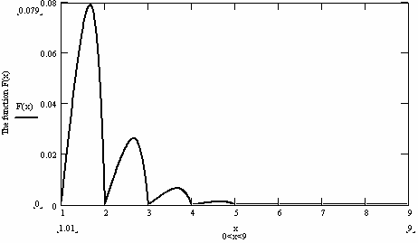
Figure 1. The Ritz Solution

Figure 5.1 gives us the visual concept of the approximate solution to the Ritz solution. The graph shows that the approximate solution is a damped oscillating function that dies out rapidly to the right.

            The Straight line on the x-axis does not guarantee the existence of a minimum value. An optimal value exists if it is unique, since the damping continues to the right ad inifitum after the fourth semi-circular curve; where the oscillating frequency dies out and becomes a straight-line almost to the base of the x-axis.

The optimized computed program code is presented below. Mathcad simulation of the problem although generates a minimum value, does not attract the conclusion of an optimum solution. The MathCad code is hereby reproduced for a pseudo conclusive result. In other words, the minimum control result presented may not be accepted as a unique output.

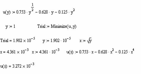
In the above computational program code, we observe that the solution to equation (5.3) is y = 1.902∙10^-2. Now from equation (4.13); x = √y; then the value of x must be x = 4.36∙10^-3. Thus, as observed, the optimized numerical value for equation (4.13) is u(x) = 3.272∙10^-3. This small numerical value constitutes an equivalence of the conjugate gradient solution to the Ritz approximate solution (4.13).

            The problem before us now is that since the graphical solution is not unique and the CGM solution does not exist, should we accept the output issued by the Mathcad computational minimum output as the final optimum result? Is the output universally acceptable as the output of our posed constraint?

Conclusions

If an optimization problem involves the minimization of a functional subject to the constraints of the same type using the Ritz algorithm or any variational methods, the decision variable will not be a number, but a function. It shows that variational methods can only give the functionals as solutions whenever a BVP is to be optimized.

Optimal control problems involve two types of variables which may be related to each other by a set of differential equations. In some obvious cases, integro-differential equations exist between the objective functions and the constraints. Lack of the explicit definition of the control and state variables in the optimal problem formulation made it difficult for us to optimize our problem using the optimal control approach. Besides, to optimize the Ritz solution, it must be converted into a dynamical constrained problem. Differentiating the Ritz solution at this point would result to creating a remarkably different problem.

By treating the Ritz approximate solution as an unconstrained equation, it is possible to solve it numerically by the Conjugate Gradient Method. This is subject to the fact that the control operator so obtained from the variational solution is a square symmetric positive definite matrix; otherwise, the optimal minimum value does not exist and we can back out from further computational labour.

We must state, however, that if the approximating terms are not wisely chosen to be of second order, using the CGM algorithm will pose difficult problems in the acquisition of the numerical value of the Ritz approximate solutions. Hence, any Ritz approximate solutions higher than the second order would be difficult to optimize using the CGM algorithm. At this state, we suggest that an ECGM (different from that of Ibiejugba and Onumanyi (1984)) be developed. The New ECGM should enable us solve any approximate Ritz solutions numerically; and or, any variational solutions as the need may arise in the computational processes.

            X-Y graphical plots of Ritz approximate solutions could be applied to give us suggestive physical interpretation of the characteristics of the variational solution to the optimal control. If the minimum value does not exist as shown on the graph, then we can not approximate it by the CGM algorithm subject to the operator being squared positive definite. Therefore, when the problem can not be extremized using the CGM algorithm, program codes could be applied as done in our work. These codes as in Mathcad program constitute the conjugate gradient optimization. Equivalent codes could be extended to non-quadratic Ritz Solutions for optimal outputs.

Most of the Ritz methods approximate solutions based on one dimensional cases exhibit damping frequency oscillations. The two-dimensional cases could be exploited on vibrational membranes modellings. This could give credence to more impetus to engineering computational methods in vibrations of mechanical components and simulates (Weaver et al (1974)).

References

[1]     Adeboye K. R., H¹-Galerkin-Collocation and Quasi-iterative Method for boundary value problem, Abacus 1997, 25, p. 286-300.

[2]     Adeboye K. R., A super convergent H²-method for the solution of two-point boundary value problems, NJTR 2002, 1, p. 36-39.

[3]     Gilbert S., George J. F, An analysis of the finite Element Method; Prentice Hall series in automatic computations, 1973.

[4]     Hasdorf L., Gradient Optimization and nonlinear control, John Wiley and Sons; 1976.

[5]     Hestenes M. R., Stiefel E., Methods of Conjugate Gradients for solving linear systems, J. Res NBS 1952.

[6]     Ibiejugba M. A., Onumanyi P., On control operators and some of its applications, J. Maths Applications 1984, 103, p. 31-37.

[7]     Jain M. K, Numerical Solutions for differential equations, John Wiley and Sons LTD, 1984.

[8]     Lambert J. D., Numerical Methods for Ordinary differential equations; the initial value problem, Wiley and Sons LTD, 1993.

[9]     Rao S. S., Optimization theory and Application, Wiley Eastern Limited, 1978.

[10]   Richard L., Burden, Faires, Douglas J., Numerical Analysis, Youngstown State University, PWS-Kent publishing Company, Boston, 1988.

[11]   Waziri V. O., Optimal control of Energized wave equations using the Extended Conjugate Gradient Methods, Ph.D. Thesis, Federal University of Technology, Minna, Nigeria; 2004.

[12]   Weaver W. (Jr.), Young D. H, Timoshenko, Vibration problems in Engineering, John Wiley and sons, 1974.