The Optimal Control of Second Order Quasi-Linear Equipotential Flows
Victor Onomza WAZIRI and Kayode Rufus ADEBOYE
Mathematics/
Computer Science Department, Federal
dronomzawaziri@yahoo.com, professorkradeboye@yahoo.com
Abstract
This research studies the optimal control of Laplacian group of equations of the second differential order and quasilinear or first degree equations in nature. The study categorizes the research into one- through to the nth-dimensional cases as points of generalization. The numerical values and physical Simulates give visual conceptions of the one-to three-dimensional equipotential flows.
Keywords
Equipotential flows;
Introduction
The Laplacian group of equations is generally categorized as equipotential flow equations. These equations give rise to elliptic partial differential equations of various dimensional cases (Hobson et al, 2002). The Laplacian equation of the second order quasilinear form is defined as:
|
|
(1.1) |
The three-dimensional equation (1.1) holds for steady temperature in isotropic medium, which characterizes gravitational or electrostatic potentials at points of empty space, and describes the velocity potential of irrotational, and or, incompressible fluid flow. Equation (1.1) is the prototype of a singular equation of the three-dimensional Laplace equation. Other dimensional singular equations cases are:
|
|
(1.2) |
|
|
(1.3) |
|
|
(1.4) |

Equations (1.2), (1.3) and (1.4) are respectively of one-, two- and the nth-dimensional quasilinear second order equipotential flow equations. We intend to obtain in this research the optimal control of these first degree equipotential flow equations using the maximum principle.
The necessary conditions for the optimal control
The necessary conditions for optimalties are clearly expunged in (Gottfried and Weisman, 1973) and (Singh and Titli, 1978) under variational expositions; but these necessary conditions for acquiring the optimal control are simplified in detail by (Rao, 1978). In a nutshell, we outline this method vis-à-vis albeit in summary as by Singh and Titli (ibid):
Consider the problem of minimizing
|
|
(2.1) |
subject to the dynamical constraint equation:
|
x(t) = f(x(t), u(t), t)) |
(2.2) |
with initial and boundary condition
|
x(t0) = x0 |
(2.3) |
These set of equations (2.1) and (2.2) yield the Hamiltonian functional in a more compact form:
|
H(x(t), u(t), λ(t)) = g(x(t), u(t), t) + λT(f(x(t), u(t),t)) |
(2.4) |
from which the necessary conditions for optimalties are derived by these statements of expressions:
|
|
(2.5) |
|
|
(2.6) |
|
|
(2.7) |
for all tÎ[t0, tf].
Furthermore, the variational approach state is defined as:
|
|
(2.8) |

Singh et al (ibid) viewed equations (2.5), (2.6) and (2.7) as the necessary conditions for optimality and containing 2n first order differential equations (that is, they consists of n state and n costate equations) and m algebraic relations (for the control equation 2.7) which need to be satisfied over the optimization period Î[t0, tf]. To solve these equations, we require 2n boundary conditions, n of these are given by the initial conditions on the state by equation (2.3) and additional n or (n+1) relationships depending on whether tf is specified. If specified and the nature of the given objective is defined as in equation (2.1) then, the additional (n+1) relationship is expressible as given by this set of combined equations (2.9) hereunder:
|
|
(2.9) |

Equation (2.4) gives the root to the formulations of the necessary conditions for optimality of a given integral quadratic objective functional. The necessary condition for optimality defined by the control equation (2.7) gives raise to the celebrated maximum principle.
Statements of the problems
In this section, we have these optimization set of problems for various equipotential second order quasilinear dimensional cases. We shall obtain their individual optimal controls in the next section using the theory in the previous section:
Problem (P1)
Optimize
|
|
(3.1) |
subject to:
|
|
(3.2) |
with initial and boundary conditions
|
z(0, t) = 0: 0 ≤ t ≤ 1 z(x, 0) = z(x): 0 ≤ x ≤ 1 |
(3.3) |
The set of equations (3.1), (3.2) and (3.3) gives the one-dimensional equipotential flow optimization problem; while in (3.2),
the additional term ![]() refers to the control at point x
and time t to a one-dimensional trajectory flow of the problem.
refers to the control at point x
and time t to a one-dimensional trajectory flow of the problem.
Problem (P2)
Optimize
|
|
(3.4) |
subject to:
|
|
(3.5) |
with initial and boundary conditions:
|
z(0, y, t) = z(x, 0, t): 0 ≤ t ≤ 1 z(x, y, 0) = z(x, y): 0 ≤ x ≤ 1, 0 ≤ y ≤ 1 |
(3.6) |
The set of equations (3.4), (3.5) and (3.6) gives the two-dimensional equipotential flow optimization control problem.
Problem (P3)
Optimize
|
|
(3.7) |
subject to:
|
|
(3.8) |
with initial and boundary conditions
|
z(0, y, w, t) = z(x, 0, w, t): 0 ≤ t ≤ 1 z(x, y, w, 0) = z(x, y, w): 0 ≤ x ≤ 1, 0 ≤ y ≤ 1 |
(3.9) |
The set of equations (3.7), (3.8) and (3.9) gives the three-dimensional equipotential flow optimization problem.
Problem (Pn)
The nth-dimensional optimizing problem is:
|
|
(3.10) |
subject to:
|
|
(3.11) |

with initial and boundary conditions
|
z(0, y, w, …, p, t) = z(x, 0, w, …, p, t) = z(x, y, w, …, 0, t) 0 ≤ t ≤ 1 z(x, y, w, …, p, 0) = z(x, y, w, …,p) 0 ≤ x ≤ 1, 0 ≤ y ≤ 1, 0 ≤ w ≤ 1, ..., 0 ≤ p ≤ 1 |
(3.12) |
We shall obtain the optimal solutions of the defined problems in the next section using the outlined theoretical computational procedures in section three above.
The computational solutions for the problems above
We divide this section into subsections according to the problems before us.
The one-dimensional second order quasilinear equipotential problem
Recall equations (3.1) and (3.2), the Hamiltonian functional is a penalized unconstrained equation of the form:
|
H(x, u, λ, t) = z2(x, t) + u2(x, t) + λ(t)[zxx(x, t) + u(x, t)] |
(4.1) |
The necessary conditions for optimal ties are defined in this sequential order:
|
|
(4.2) |
|
|
(4.3) |
|
|
|
that is:
|
λ = -2u(x, t) |
(4.4) |
Differentiating equation (4.4) and comparing its output with that of equation (4.2), yields a first order partial differential equation of the form:
|
|
(4.5) |
In a characteristic procedure as in Zachmann and Duchateau (1986), if equation (4.5) has a Fourier series solution, then set
|
|
(4.6) |
|
|
(4.7) |
Differentiating (4.6) with respect to t gives:
|
|
(4.8) |
implying that
|
αi = uit |
(4.9) |
Thus constraint equation (3.2) could be expressed as:
|
|
(4.10) |
such that the characteristic equation (4.10) is defined as
|
-i2π2λ + 1 = 0 |
|
therefore, the characteristic root λ is comparable as:
|
|
(4.11) |
The quadratic objective functional (3.1) is expressible as:
|
|
(4.12) |
subject to the general sequential characteristics solutions:
|
|
(4.13) |
Equation 4.13 yields the general characteristic expressions:
|
-22π2λ + 1 = 0 |
(4.14) |
|
…………………………. |
|
|
-i2π2λ + 1 = 0 |
(4.15) |
The corresponding unconstraint minimization problem is succinctly defined as:
|
|
(4.16) |
Now solving the ![]() equation (4.13) by suppressing the
independent variable x yields
equation (4.13) by suppressing the
independent variable x yields
|
u(.,t) + aeλt |
(4.17) |
It then follows
from equations (4.6) and (4.17) and with![]() , that:
, that:
|
|
(4.18) |
Hence, with equation (4.17) and with considerations of equations (4.11) and (4.18), the general solution to equation (4.13) is:
|
|
(4.19) |
Furthermore, from the computational derivations above, we observe that the partial derivative of the control u(x, t) with respect to t is the state z(x, t). Thus from equation (4.19), the state equation is defined in this order:
|
|
(4.20) |
Therefore for the one-dimensional quasilinear equipotential flow equation, the control and state are equations (4.19) and (4.20) respectively.
The two-dimensional second order quasilinear equipotential flow optimization problem
In a systematic manner as above, it would not be difficult to derive the optimal control and state to the two-dimensional problem.
The Hamiltonian form is:
|
H = z2(x, y, t) + u2(x, y, t) + λT(zxx(x, y, t)) + zyy(x, y, t) + u(x, y, y) |
(4.21) |
The necessary conditions for optimality are given as:
|
|
(4.22) |
|
|
(4.23) |
|
|
(4.24) |
Comparing equations (4.22) and (4.23), we have the first order quasilinear equation:
|
|
(4.25) |
As in the above, the assuming a Fourier series solution:
|
|
(4.26) |
with the state defined as:
|
|
(4.27) |
From equations (4.26) and (4.27), we have the constraint equation (3.5) transformed to:
|
|
(4.28) |
Equation (4.28) maybe simplified and written in a characteristic formulation as:
|
2i2π2λ2 – 1 =0 |
(4.29) |
Without following the necessary rewriting the minimizing procedures, we have:
|
|
(4.30) |
Solving equation (4.28), we have the optimal control as
|
|
(4.31) |
In the same manner as in one-dimensional case, the state is defined as:
|
|
(4.32) |
Equations (4.31) and (4.32) are the desired optimal control and state functional respectively.
The optimal control and state for the three-dimensional equipotential flow
Without much ado, it will not have us confused to generalize from the two subsections of this section that the optimal control and state equations are defined sequentially as:
|
|
(4.33) |
|
|
(4.34) |
Equations (4.33) and (4.34) are the respective three-dimensional optimal control functional solutions.
The optimal control and state for the n-dimensional equipotential flow
Following the same pattern as the three subsections, we conclude that the optimal control and state mth-dimensional optimization problem are easily invoked as in these observations:
|
|
(4.35) |
|
|
(4.36) |
With the derived various optimal control and state functional solutions, we now obtain the numerical values of each dimensional space. We envisage tremendous difficulty in simulating the physical optimal control and state for the visual conception of any higher dimensional spaces greater than three-dimensional case. Thus our analysis is on the one- through to the three-dimensional derivations cases above.
The optimal numerical analysis
We obtain the following numerical values for the following dimensional problems:
The one-dimensional problem program outputs are
The optimal numerical solution outputs using program code for the one-dimensional case are: u(x, t) = 3.927∙10-4 and z(x, t) = 1.591∙10-6 for the optimal control respectively. These are achieved when x = -0.019 at t = 1.943∙104.
The two-dimensional numerical optimal outputs
The optimal numerical values outputs using program codes are as follow:
The optimal control u(x, y, t) = 2.468∙10-9 and state z(x, y, t) = 1.25∙10-10 are obtained when n = 1, x = 2.5∙10-5, y = 5∙10-5, and t = 2.5∙10-4.
The three-dimensional numerical optimal values
The three-dimensional case is quite revealing as shown below; for as the dimensional space is increased; both the optimal control and state output become progressively small as demonstrated in this numerical output. The optimal control at this space is u(x, y, w, t) = 1.938∙10-11 while the state trajectory is z(x, y, w, t) = 6.545∙10-13.
These optimal numerical values are obtained when n = 1, x = 2.5∙10-5,y = 5∙10-5, w = 6.25∙10-5, and t = 5∙10-5.
Remarks on numerical observations
The observations made so far, manifest an increase in potential energy with consequent advancement in dimensional space. The analogy is significant if we compare the numerical wavelengths in the control and state as related to the one- and two-dimensional cases; or two-dimensional and three-dimensional optimal results observations. Hence higher frequencies manifestations would be observed with attendance of shorter wavelengths.
This study revealed some fundamental theoretical truths that the higher the concentration of matter at the centre (henceforth referred to as epicentre), the epicentre becomes more excited in agitations due to enormous experience of higher potential energy.
Following this traditional acquisition of the numerical optimal values, we can go ad-inifinitum to obtain various dimensional equipotential flows control and state numerical values at various increasing variables sequentially as the dimensions are increased step wisely.
We note in passing, however, that the optimal numerical values (which represent wavelengths values) become infinitesimal as the dimensional spaces enlarged. Furthermore, we state in passing that the exhibited wavelength numerical values vary with an increase in mth-plane profile.
The Simulates of the one- to three-dimensional spaces
Here, we give the physical simulates of the three functional solution spaces as derived in subsections of section 4 above when n=1.
The one-dimensional Simulate for the states and controls are as follows:
The one-dimensional case
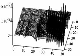
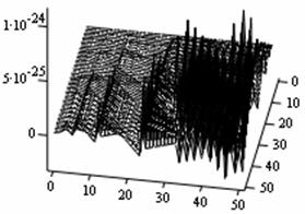
Figures 1 and 2 are the optimal control and state Simulates for the one-dimensional equipotential flows respectively. Both exhibit plains central regions; but the edges are rather overwhelmed with much wave turbulences in separated fashions. The Amplitudes are more conspicuous outwardly into our chests and in varied amplifications to the right for optimal control and to the left by the optimal state.
|
u |
z |
|
Figure 1. Optimal control simulate at n = 1 |
Figure 2. optimal state simulate at n = 1 |
The two-dimensional case
Figures 3 and 4 represent the Simulates for the two-dimensional space. The wave disturbances are more turbulent than the one-dimensional cases above. The relative peaceful plain in the one-dimensional case has conspicuously disappeared here. This maybe attributed to their differences in the wavelengths; their optimal numerical comparisons buttress this assertion.
|
|
|
|
Figure 3. Optimal control at n = 1 |
Figure 4. Optimal state at n = 1 |
The Simulates for three-dimensional
In a similar examinations as above, we have the control and state Simulates in figures 5 and 6 respectively for the three-dimensional case. The wave forms are more compact and with shorter wavelengths here than in the previous observations. This spectacular observation portents greater energy potential differences than the two previous assessments.
|
u |
z |
|
Figure 5. Optimal control at n = 1 |
Figure 6. Optimal state at n = 1 |
Conclusions
The research work has been quite illuminating. The computational numerical values show that the higher the dimensional space, the smaller are the numerical optimal control and state values. These diminishing numerical values demonstrate to some extend that the energy packages in the higher dimensional spaces are more significant than in the lower spaces. That is, energy experienced by a one-dimensional equipotential flow space equation is less than that experienced by two-dimensional case and so on. The observed Simulates clearly give weight to the aforementioned observations. As the Simulates dimensional spaces increase, their physical observations exhibit some compact wave patterns with shorter optimal controls and states wavelengths. What this compactness portrays is that the higher the dimensional space of an equipotential flow, the higher is the energy level; which symbolizes a high attendance of frequencies observations.
Another prominent observation made is that the mth-profile change in space. The mth-value describes here simply refer to the mth-plane stratum. These strata give raise to differences in the equipotential energy levels even in the same dimensional space. Thus energy levels at the epicentre of any equipotential flows are higher than those within their neighbourhood. This accounts for the theoretical belief that the centre of the earth has much more energy package than its neighbourhood which reduces in quantity as one move away from its epicentre.
We must state that the application of our findings to the forgone analytical discourse presumes free-gravitational space within the earth interior.
References
1 Duchateau P., Zachmann D. W., Partial differential equations, McGraw-Hill Publishing company, 1986.
2 Gottfried B. S., Weisman J., Introduction to optimization theory, Prentice-Hall, Englewood Cliffs, New Jersey, 1973.
3 Hobson M. P, Riley K. F., Bence S. J., Mathematical Methods for Physics and engineering, Cambridge University Press, 2002.
4 Hughes F. W., Brighton J. A., Fluid Dynamics with an introduction to subsonic and Supersonic flow incompressible Turbulent flow Hypersonic boundary layer flow Magnetodrodynamics Non-Newtonian Fluids, International Editions; Schaum’s Outline series, 1991.
5 Ibiejugba M. A., On Krassnoselskiii’s moment inequality, Advances in Modelling and Simulations 1987, 6(3), p. 1-17.
6 Lambert J. D., Numerical Methods for ordinary Differential systems, John Wiley and Sons, 1993.
7 Rao S. S., Optimization Theory and Application, Wiley Eastern Limited, 1978.
8 Reju S. A., Computational Optimization in Mathematical, Ph.D. Thesis, University of Ilorin, Ilorin, Nigeria, 1995.
9 Reju S. A., Ibiejugba M. A., Evans D.J., Computational Results of the Optimal Control of the diffusion Equation with the Extended Conjugate Gradient Problem, Advances in Modelling & Analysis 1999, 3(2), p. 1-22.
10 Reju S. A., Ibiejugba M. A., Evans D. J., Optimal Control of the Wave Propagation Problem with the Extended Conjugate Gradient Method, Inter. J. Computer Math., 2001, 77(3), p. 425-439.
11 Singh M. A., Titli A. J., System Decomposition, Optimization and Control, Pergason Toulouse, France, 1978.
12 Smith G. D., Numerical Solution of partial Differential equations: Finite Difference Methods, Oxford University Press, 1985.
13 Waziri V. O., Optimal control of Energized Wave equations using the Conjugate Gradient method, Ph.D. Thesis, Federal university of Technology, Minna, Nigeria, 2004.