Modeling of Static Series Voltage Regulator (SSVR) in Distribution Systems for Voltage Improvement and Loss Reduction

 

Mehdi HOSSEINI ^1*, Heidar  Ali SHAYANFAR¹, Mahmoud FOTUHI-FIRUZABAD²

 

¹Center of Excellence for Power System Automation and Operation, Department of Electrical Engineering, Iran University of Science & Technology, Tehran, Iran

²Sharif University  of Technology, Tehran, Iran

^*Corresponding author. E-mail: mehdi_hosseini@iust.ac.ir

 

 

Abstract

This paper introduces the modeling of Static Series Voltage Regulator (SSVR) in the load flow calculations for steady-state voltage compensation and loss reduction. For this approach, an accurate model for SSVR is derived to use in load flow calculations. The rating of this device as well as direction of required reactive power injection to compensate voltage to the desired value (1^p.u.) is derived, discussed analytically, and mathematically using phasor diagram method. Since performance of SSVR varies when it reaches to its maximum capacity, modeling of SSVR in its maximum rating of reactive power injection is derived. The validity of the proposed model is examined using two standard distribution systems consisting of 33 and 69 nodes, respectively. The best location of SSVR for under voltage problem mitigation and loss reduction in the distribution systems is determined, separately. The results show the validity of the proposed model for SSVR in large distribution systems.

Keywords

Distribution System; Static Series Voltage Regulator (SSVR); Voltage Compensation; Loss Reduction; Load Flow.

Abbreviations

RUVMN = Rate of Under Voltage Mitigated Nodes.

 

 

1. Introduction

 

The main purpose of this paper is the effect of SSVR on the voltage compensation as well as loss reduction in distribution systems. In the presented papers in the literature, shunt capacitor and reconfiguration are generally used in radial distribution systems for loss reduction emphasizing on the active power losses i.e. RI² [1-3]. In this paper the effect of SSVR on both active (RI²) and reactive losses (XI²) is considered. There are two principal conventional means of controlling voltage on distribution systems: series voltage regulators and shunt capacitors. Conventional series voltage regulators are commonly used for voltage regulation in distribution systems [4-6]. These devices are not capable to generate reactive power and by its operation only force the source to generate reactive power. Furthermore, they have quite slow response and their operations are step-by-step [7]. Shunt capacitors can supply reactive power to the system. Reactive power output of a capacitor is proportional to the square of the system voltage that its effectiveness in high and low voltages may be reduced. Hence, for improvement of capacitors in different loading conditions, their constructions are generally combined of fixed and switched capacitors. Therefore, they are not capable to generate continuously variable reactive power. Another difficulty associated with the application of distribution capacitors is the natural oscillatory behavior of capacitors when it is used in the same circuit with inductive components. This sometimes results in the well-known phenomena of ferroresonance and/or self-excitation of induction machinery [7]. Hence, when regulators that operate by adjusting their taps to maintain predetermined set point voltage levels are coupled with capacitors that are switched on and off to regulate voltage, the voltage swings can cause power quality problems for customers.

With the improvements in current and voltage handling capabilities of the power electronic devices that have allowed for the development of Flexible AC Transmission System (FACTS), the possibility has arisen in using different types of controllers for efficient shunt and series compensation. It should be noted that FACTS devices respond quickly to the changes in network condition. The concept of FACTS devices was originally developed for transmission systems, but similar idea has been started to be applied in distribution systems. Dynamic Voltage Restorer (DVR) is a series connected converter which is used to compensate some of the power quality problems such as voltage sag, voltage unbalance
[8-13] which occurs in short duration in millisecond range. In this duration, DVR can inject both active and reactive power to the system for compensation of sensitive loads and active power injection into the system must be provided by energy storage system [8]. Almost, all of the models reported for DVR have been utilized in a two-bus distribution system consist of a sensitive load and the source. Then, effects of DVR modeling on compensation of power quality problems of sensitive loads have been considered. However, the effects of DVR on
large distribution system and other loads in the distribution systems have not been considered. Also, the impacts of DVR are dynamically considered in a short duration but not considered for a long term. In this work, effect of series distribution FACTS device on loss reduction and static voltage regulation is considered. It is therefore proposed that its name should be a Series Static Voltage Regulator (SSVR).

In this paper, SSVR is used for the voltage improvement and loss reduction in long term applications. Since this device is utilized in steady-state condition for a long term, because of limited capacity of energy storage system, it can not inject active power to the system. Therefore, suitable model for SSVR has been proposed in load flow program that is applicable in large distribution systems. In addition, the rating and direction of reactive power that must be exchanged by SSVR for voltage compensation in desired value (1p.u.) is derived and discussed as analytically and mathematically using phasor diagram method. Moreover, modeling of SSVR in its maximum rating of reactive power injection is derived and mathematically expressed. Then, effects of SSVR on voltage improvement at other nodes and also loss reduction in the distribution system are considered. The best location of SSVR for under voltage problem mitigation and loss reduction is determined, separately. Two standard distribution systems consist of 33 and 69 nodes are considered and SSVR model is applied in load flow. The results reveal the effectiveness of the proposed model for the SSVR in large distribution systems.

Section 2 presents steady-state modeling of SSVR. In section 3, radial distribution system with load flow method has briefly been discussed. Model of SSVR on load flow is represented in section 4. In section 5, the results associated with application of SSVR model on 33-bus and 69-bus standard distribution systems are presented and discussed. Finally, section 6 summarizes the main points and results of this paper.

 

 

2. Steady-State Modeling of Static Series Voltage Regulator (SSVR)

 

2.1. Static Series Voltage Regulator (SSVR)

 

Dynamic Voltage Restorer (DVR) is a series device used to add a voltage vector to the network to improve the quality of the voltage supplied by the network. The main function of DVR is to eliminate or to reduce voltage sags, phase unbalance and harmonics of the supply seen by the sensitive load. Voltage sag occurs in less than 1 minute within which DVR can inject both active and reactive power for voltage correction. Injection of active power into the system must be provided by energy storage system (Fig. 1). Small voltage sags can usually be restored through reactive power only but for larger voltage sags, it is necessary to inject active power into the system by DVR to correct the voltage sags.

Figure 1. A typical model of DVR

 

Because of limited capacity of energy storage system, it cannot inject active power to the system for long term voltage regulation. Energy storage system must therefore be replaced with dc capacitor for long term applications. Thus, in the steady-state application, series compensator consists of dc capacitor and voltage source converter. In this paper, we focus on the effect of series compensator on loss reduction and static voltage regulation in a steady-state condition. It is therefore proposed that its name should be a Static Series Voltage Regulator (SSVR). A typical model of SSVR is shown in Fig. 2. Control system in SSVR acts as the steady-state power exchange between SSVR and the network is reactive power, in other words, injected voltage by voltage source converter in SSVR must be kept in quadrate with .

Figure 2. A typical model of SSVR and phasor diagram of reactive power exchange operation

 

 

2.2 Steady-State Modeling of SSVR

 

The single line diagram of two buses of a distribution system and it is phasor diagram are shown in Fig. 3 and Fig.4, respectively. Generally, voltage of buses in the system is less than 1^p.u. and it is desired to compensate voltage of interested bus j () to 1^p.u. by using SSVR. In Fig. 3, the relationships between voltage and current can be written as:

(1)

where:

	voltage of bus j before compensation
	voltage of bus i before compensation
	impedance between buses i and j
	current flow in line before compensation

 

Voltages  and and current are derived from load flow calculations.

Figure 3. Single line diagram of two buses of a distribution system

Figure 4. Phasor diagram of voltages and current of the system shown in Fig. 3

 

In this section, injected voltage by SSVR and new angle of compensated voltage are derived as voltage magnitude in bus j changes from  to 1^p.u. in the steady-state condition. By installing SSVR in distribution system, all nodes voltage, especially the neighboring nodes of SSVR location, and braches current of the network change in the steady-state condition. The schematic diagram of buses i and j of a distribution system when SSVR is installed for voltage regulation in bus j is shown in Fig. 5. Since SSVR is used for voltage regulation in the steady-state condition, it can inject only reactive power to the system. Therefore,  must be kept in quadrature with current flow of SSVR, i.e.. Using SSVR, voltage of bus j changes from  to  as shown in the phasor diagram of Fig. 6. For the sake of simplicity, the angle of voltage, i.e.,   is assumed to be zero in phasor diagrams. It can be seen from Fig. 5 and Fig. 6 that:

 

Figure 5. Single line diagram of two buses of a distribution system with SSVR consideration

 

Figure 6.  Phasor diagram of voltages and current of the system shown in Fig. 5

 

	(2)
	(3)

where:

	Voltage of bus j after compensation by SSVR
	Voltage of bus i after compensation by SSVR
	Current flow in line after SSVR installation
	Injected voltage by SSVR

 

Voltage  and current  are derived from the load flow calculations.

Separating the real and imaginary parts of equation (2) yields to:

(4)

and:

(5)

 

Equations (6) and (7) are obtained from equations (4) and (5), respectively by considering the following assumptions:

 

	(6)
	(7)

where,,,and are constants and  is the magnitude of compensated voltage (1^p.u. ) and ,are variables. Rearranging equation (6) and (7) yields to:

(8)

and:

(9)

Considering that:

(10)

then:

(11)

Therefore:

(12)

where:

Two roots for  are derived out of which one of them is acceptable. To determine the correct answer, these roots are examined under the following boundary conditions below in the load flow results:

'' if  then ''

 

After testing these conditions on the load flow results, correct answer for  is selected as:

(13)

Then, using equations (14) or (15),  can be defined as shown below:

(14)

or:

(15)

Finally, injected reactive power by SSVR can be expressed as:

(16)

where:

where, the symbol " * " denotes conjugate of complex variable.

 

2-3. Modeling of SSVR in its Maximum Rating of Reactive Power Injection

It is assumed that the voltage magnitude in node j, i.e. , is considered to the specified value, i.e. b (for example 1^p.u.). Then, phase angle of voltage in node j, i.e. , and injected voltage and reactive power by SSVR are derived from (14), (13) and (16), respectively. However, when calculated reactive power by (16) is greater than the maximum reactive power rating of SSVR, maximum magnitude of injected series voltage by SSVR can be expressed as below:

(17)

On the other hand, the phase angle of injected series voltage by SSVR can be determined from (3). Therefore, the injected voltage by SSVR in this case can be expressed as below:

(18)

Under this condition, the magnitude of compensated voltage can not be regulated in the specified value (for example 1^p.u.). Therefore, new voltage magnitude () and phase angle )) of compensated node j are calculated using rearrangement of  (2) as:

(19)

 

 

3. Radial Distribution Systems Load Flow

 

Load flow is an important and basic method for analysis, operation and planning studies of any power system in a steady-state condition. By using load flow, it can be determined that which variables exceed their limits and thus efficient corrective solutions such as shunt, series and other compensation techniques must be taken to stir the state variables within an acceptable and secured operating zone. Most distribution systems are fed at one point and system has a radial structure. Several methods have been developed for radial distribution systems [14-16]. An efficient and simple load flow method based on backward/forward sweeps is used in this paper and is described below [16].

 

3.1. Load Flow Equations

It is assumed that the three-phase radial distribution system is balanced. The single line diagram of two buses of a given distribution system is shown in Fig. 7.

Figure 7. Single line diagram of two buses of a distribution system

 

Based on node and branch numbering, voltage of node i can be expressed as:

(20)

where:

	Voltage of node i
	Voltage of node i-1
	Impedance of line i
	Current flow in line i

Since the voltage of source node is known, equation (20) can be used in forward sweep to determine voltage of other nodes in distribution systems.

The load current of node i,, can be written as:

(21)

where and are respectively active and reactive power of the load connected to node i.

The current through branch i,  is equal to load current of node i,, plus the sum of the branch currents which are connected to this line, i.e.:

(22)

where, set  consists of all branches which are connected to node i. Node i is designated as an end node for which set  is empty and therefore, current through branch i which is connected to the end nod i can be expressed as:

(23)

Total active and reactive power loss in the distribution system can be written as the following equations:

 

(24)

 

(25)

 

where, nb is the number of distribution system branches.

 

3.2. Backward/Forward Sweeps in Load Flow and Convergence Criterion

Initially, a constant voltage of all nodes is assumed to be (). Then all load currents are computed using equation (21). After that, branch currents are computed using equations (22) or (23) in backward sweep. Thereafter, voltage of each node is calculated using equation (20) in forward sweep. Once the new values of voltages of all nodes are computed, convergence criterion of the solution is checked. If it does not converge, then load currents are computed using the most recent values of voltages and the whole process is repeated. The convergence criterion is that, in successive iterations the maximum difference in voltage magnitudes must be less than 0.0000l ^p.u..

 

 

4. Modeling of SSVR in Load Flow

 

As mentioned before, SSVR is a series device that injects a series voltage to the distribution system to improve voltage of interested node in the steady-state condition. Therefore, for modeling of SSVR in any iteration of load flow in forward sweep, at first, it is assumed that the voltage magnitude of the compensated node is 1^p.u.. Then, the phase angle of compensated voltage and rating of injected reactive power by SSVR are calculated from equations (14) and (16), respectively. If calculated reactive power is greater than the maximum reactive power rating of the SSVR, the magnitude and phase angle of compensated voltage are derived from (19) and injected reactive power by SSVR must be set to its maximum rating. Then, in the forward sweep of the load flow, new magnitude and phase angle of compensated node are utilized to determine voltage of SSVR location down stream nodes. Then, updated voltages of nodes are used for the determination of load currents using equation (21) in the next backward sweep. These processes are continued until the load flow is converged.

 

 

5. Simulation Results

 

Two distribution systems consisting of 33 and 69 buses are selected and the proposed models associated with SSVR are used to examine the applicability of SSVR and illustrate the proposed approach. The results obtained in these systems are briefly summarized in the following sections.

 

5.1. 33-Bus Test System

The single line diagram of the 12.66 kV, 33-bus, 4-lateral radial distribution system is shown in Fig. 8. The data of the system are obtained from [2]. The total load of the system is considered as (3715+ j 2300) kVA. A summery of load flow solution before SSVR installation is presented in Table 1. It is assumed that the upper and lower limits of voltage magnitude are 1.05 ^p.u. and 0.95 ^p.u., respectively. It can be seen that 21 nodes out of 33 nodes of the distribution system (63.63 %) have under voltage problem. In this system active and reactive power loss are 202.68 kW and 135.19 kVAr, respectively.

In order to illustrate and compare the effects of SSVR implementing in the distribution system, different locations are selected for installation of SSVR. For this purpose, nodes 17 and 32 as the end nodes, nodes 12 and 28 in the laterals, and nodes 3 and 5 in the main feeder of the distribution system are selected. In fact, SSVR is utilized to compensate voltage at the selected nodes to 1^p.u. and to improve voltage of other nodes in the system. Moreover, the effect of SSVR on loss reduction in the distribution system is considered. Also, effect of capacity constraint in SSVR for voltage compensation and loss reduction is studied and compared to the case that it has no capacity limit. It should be noted that only one SSVR is used at a time while performing load flow calculations.

 

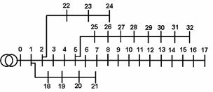
Figure 8. Single line diagram of 33 bus distribution system

 

Table 1. Voltage magnitude and phase angle in 33 bus distribution system without implementing SSVR

 

Table 2 shows the result of load flow calculations with SSVR consideration for compensation of voltage in the selected nodes. It is observed from Table 2 that when SSVR is installed in each line of the distribution system, only the voltage of the downstream
nodes is improved, whereas that of the upstream nodes is slightly improved. For example, by installing an SSVR in line 32, in order to compensate voltage at node 32 (the end node), only the voltage of node 32 is improved and regulated at 1^p.u. while the voltage of other nodes are affected rarely. In other words, SSVR installation in line 32 mitigates under voltage problem of only one node out of 33 nodes (3.03 %). Similarly, the same results are achieved by SSVR installation in line 17 (Table 2). In the next stage of simulation, the effect of SSVR installation in the laterals of the distribution system is considered. For this purpose, an SSVR is installed in the line 12 for voltage compensation at node 12. The results show that SSVR installation in this line strongly improves the voltage of neighboring downstream nodes (13, 14, 15, 16 and 17) and therefore mitigates under voltage problem of these nodes. Furthermore, the voltage of upstream nodes is slightly improved. For example, only voltage of node 5 (an upstream node) is compensated from 0.9497 ^p.u. (Table 1) to 0.9509 ^p.u. (Table 2) and its under voltage problem is mitigated. Similar result is obtained by SSVR installation in line 28. Afterwards, the effect of SSVR installation in the main feeder of the distribution system is investigated.

 

Table 2. Voltage magnitude in 33 bus distribution system with SSVR consideration

 

It is observed from Table 2 that when SSVR is installed in line 5, under voltage problem in all nodes are mitigated. Also, the effect of SSVR installation on voltage improvement and loss reduction in each line of the distribution system is studied and the results are shown in Table 3. This table includes Rate of Under Voltage Mitigated Nodes (RUVMN), amount of active and reactive power loss reduction and injected reactive power by SSVR. The plus sign for reactive power rating of SSVR indicates that the injected voltage by SSVR leads by 90º with respected to its current. From the voltage profile improvement viewpoint, SSVR installation in lines 21, 24, 17, and 32 for voltage compensation respectively at nodes 21, 24, 17, and 32 (the end nodes), has a small effectiveness in the distribution system. Also, SSVR installation for voltage compensation at nodes 18, 19, 20, 21, 22, 23 and 24 can not improve voltage of the other nodes significantly. The reason for this is that voltage at these nodes are within limits before installation of SSVR (Table 1) and moreover are located far from the under voltage nodes. Based on the results shown in Table 3, the best location for SSVR installation for under voltage mitigation is line 5 because RUVMN is 63.63% in this location. Furthermore, from the loss reduction viewpoint, SSVR installation in the distribution system can reduce both active and reactive power loss. From Table 3, it is observed that SSVR installation in lines connected to the end nodes i.e. 21, 24, 17, and 32 has a small effect on loss reduction. Based on the results of Table 3, the best location for SSVR installation for loss reduction is line 5 reducing 17.12 kW and 11.72 kVAr of active and reactive power loss, respectively.

 

Table 3. Rate of Under Voltage Mitigated Nodes (RUVMN), amount of active and reactive power loss reduction and injected reactive power by SSVR in 33 bus distribution system

 

The results of Tables 2 and 3 are achieved based on the assumption that SSVR has no capacity limit for reactive power injection to voltage compensation. In order to study the effect of capacity constraint in SSVR, it is assumed that the maximum injected reactive power by SSVR is 75 kVA. Table 4 shows that the ability of SSVR in voltage compensation and loss reduction is decreased when its reactive power rating is limited. The results show that the RUVMN is decreased in many places as compared to Table 3. In addition, the usefulness of SSVR decreases much more when the difference between required reactive power and maximum rating of reactive power of SSVR becomes greater. For example, 75 kVA SSVR installation at lines 3, 4, 5, 6 and 7 causes RUVMN decrease from 33.33% to 18.18%, 54.54% to 21.21%, 63.63% to 21.21%, 39.39% to 21.21%, and 36.36% to 21.21%, respectively. In the best case, 75 kVA SSVR can mitigate only 33.33% of under voltage problem in the system and it is achieved when it is installed in line 8. Also, the results show that the amount of reduced losses is decreased in many places as compared to Table 3. For example, installation of a 75 kVA SSVR at lines 3, 4, 5, 6, 7, 8, 9, 10 and 11, does not reduce losses of system significantly. The best location for a 75 kVA SSVR for loss reduction is line 30 reducing 7.337 kW and 5.050 kVAr of  active and reactive power loss, respectively.

 

Table 4. Rate of Under Voltage Mitigated Nodes (RUVMN), amount of active and reactive power loss reduction and injected reactive power by  75 kVA SSVR in 33 bus distribution system

 

 

5.2. 69-bus test system

 

The 12.66 kV, 69-bus, 8-lateral radial distribution system based on new node numbering with few modifications in active and reactive power demand is considered as another test system. The data of the system are obtained from [3]. The total load of the system is considered as (4.0951+ j 2.8630) MVA. New and basic node numbering is presented in Tables 5 and 6. The upper and lower limits of voltage magnitude are considered 1.05 ^p.u. and 0.95 ^p.u., respectively. A summery of load flow solution before SSVR installation shows that 18 nodes out of 69 nodes of the distribution system (26.08%) have under voltage problem. These nodes consist of the nodes with numbering from 18 to 26 and 45 to 53 (based on new node numbering). In this system active and reactive power loss are 255.65 kW and
115.88 kVAr, respectively.

Table 5 shows the results of Unlimited SSVR installation in each location of 69-bus distribution system. This table includes Rate of Under Voltage Mitigated Nodes (RUVMN), amount of active and reactive power loss reduction, and the injected reactive power by Unlimited SSVR. The plus sign for reactive power rating of SSVR indicates that the injected voltage by SSVR leads by 90º with respected to its current.

 

Table 5. Rate of Under Voltage Mitigated Nodes (RUVMN), amount of active and reactive power loss reduction and injected reactive power by Unlimited SSVR in 33 bus distribution system

Based on the result shown in Table 5, the best locations for Unlimited SSVR installation to mintage under voltage problem are lines 7, 8 and 45, respectively which have RUVMN equals to 15.94%. Moreover, the best location for Unlimited SSVR installation for loss reduction is line 49 that reduces 34.02 kW and 14.57 kVAr of active and reactive power loss, respectively. Table 6 includes Rate of Under Voltage Mitigated Nodes (RUVMN), amount of active and reactive power loss reduction, and the injected reactive power by 75 kVA SSVR. The Results of this table show that the ability of SSVR in voltage compensation and loss reduction is decreased when its reactive power rating is limited. The results show that  the best location for 75 kVA SSVR installation are lines 5, 6, 7, 8, 9, 10, 11, 2, 13, 14, 15, 16, 17, 18, 19 which have RUVMN equals to 13.04%. By installation of a 75 kVA SSVR at lines 44, 45, 46, 47, 48 and 49, the RUVMN is decreased from 10.14% to 1.449%, 15.94% to 1.449%, 14.49% to 0%, 13.04% to 0%, 11.59% to 0% and 10.14% to 0%, respectively. Furthermore, the results show that the amount of loss reduction is decreased in many places such as 6, 7, 8, 41, 42, 43, 44, 45, 46, 47, 48 and 49. The best location for a 75 kVA SSVR for loss reduction is line 51; decreasing 8.702 kW and 3.728 kVAr of  active and reactive power loss, respectively.

Totally, comparing the effect of SSVR installation in the two cases, it is concluded that the performance of this device in these two test systems and also its effectiveness are approximately similar; demonstrating the validity and effectiveness of the proposed model.

 

 

6. Conclusions

 

In this paper, model of Static Series Voltage Regulator (SSVR) in load flow program is derived. In this model rating and direction of reactive power injection designated as SSVR for the voltage compensation in desired value (1^p.u.) is derived and discussed analytically and mathematically using phasor diagram method.  Also, model of this device in its maximum
rating of reactive power injection is derived. The model of SSVR is applied in load flow calculations in 33 and 69 bus test systems. Moreover, the best locations of SSVR for under voltage problem mitigation and loss reduction approach in the test systems are derived. Also, effect of capacity limit of SSVR for voltage compensation and loss reduction in the test systems is considered. The results presented indicate that SSVR can be used for under voltage problem mitigation and loss reduction. The results also illustrate that the ability of SSVR in voltage compensation and loss reduction is decreased when its reactive power rating is limited. The results indicate the validity of the proposed model for SSVR in large distribution systems.

 

Table 6. Rate of Under Voltage Mitigated Nodes (RUVMN), amount of active and reactive power loss reduction and injected reactive power by  75 kVA SSVR in 33 bus distribution system

 

 

Reference

 

1.      Haque M. H., Capacitor placemebt in radial distribution systems for loss reduction, IEE Proc. Gener. Transm. Distrb., 1999, 146(5), p. 641-648.

2.      Baran M. E., WU F. F., Network reconfiguration in distribution systems for loss reduction and load balancing, IEEE Transactions on Power Delivery, 1989, 4(2), p. 1401-1407.

3.      Baran M. E., Wu F. F., Optimal capacitor placement on radial distribution systems, IEEE Transactions on Power Delivery, 1989, 4(1), p. 725-732.

4.      Bishop M. T., Foster J. D., Down D. A., The application of single-phase voltage regulators on three-phase distribution systems, Rural Electric Power Conference, the 38th Annual Conference, pp. C2/1-C2/7, April, 1994.

5.      Gu Z. and Rizy D. T., Neural networks for combined control of capacitor banks and voltage regulators in distribution systems, IEEE Transactions on Power Delivery, 1996, 11, p. 1921-1928.

6.      Kojovic L. A., Coordination of distributed generation and step voltage regulator operations for improved distribution system voltage regulation, IEEE Power Engineering Society General Meeting, pp. 232-237, June, 2006.

7.      Ramsay S. M., Cronin P. E., Nelson R. J., Bian J., and Menendez F. E., Using distribution static compensators (D-STATCOMs) to extend the capability of voltage-limited distribution feeders, Rural Electric Power Conference, the 39th Annual Conference, pp. A4/1-A4/7, April, 1996.

8.      Haque M. H., Compensation of distribution system voltage sag by DVR and D-STATCOM, 2001 IEEE Porto Power Tech Conference, 2001, 1, p. 223-228.

9.      Ghosh A., and Ledwich G., Compensation of distribution system voltage using DVR, IEEE Transactions on Power Delivery, 2002, 17, p.1030-1036.

10.  Ding H., Shuangyan S., Xianzhong D. and Jun G., A Novel Dynamic Voltage Restore and Its Unbalance Control Strategy Based on Spaced Vector PWM, ELSEVIER, Electric Power Systems Research 2002, 24, p.693-699.

11.  Jindal A. K., Ghosh A., Joshi A., Voltage regulation using dynamic voltage restorer for large frequency variations, IEEE Power Engineering Society General Meeting, 2005, 1, p. 850-856.

12.  Nguyen P. T., and Saha T. K., Dynamic voltage restorer against balanced and unbalanced voltage sags: modelling and simulation, IEEE Power Engineering Society General Meeting, 2004, 1, p.639-644.

13.  Meyer C., Romaus C., and De Doncker R.W., Optimized Control Strategy for a Medium-Voltage DVR, 36th IEEE Power Electronics Specialists Conference, PESC 2005, pp. 1887-1893.

14.  Haque M. H., Efficient load flow method for distribution systems with radial or meshed configuration, IEE Proc. Gener. Transm. Distrb., 1996, 143(1), p. 33-38.

15.  Jin M. A., Jianyuan X. U., Shenghui W. and XIN L, Calculation and analysis for line losses in distribution network, IEEE International Conference on Power system Technology, pp. 2537-2541, 2002.

16.  Ghosh S. and Das D., Method for load-flow solution of radial distribution networks, IEE Proc. Gener. Transm. Distrb., 1999, 146(6), p. 641-648.