Neuro-Fuzzy DC Motor Speed Control Using Particle Swarm Optimization

Boumediene ALLAOUA^*, Abdellah LAOUFI, Brahim GASBAOUI, and Abdessalam ABDERRAHMANI

Department of Electrical Engineering, Bechar University, B.P 417 BECHAR (08000) Algeria

E-mails: elec_allaoua2bf@yahoo.fr, brahim_gasb@yahoo.com, laoufi_ab@yahoo.fr, abderrahmani@yahoo.fr

^*Corresponding author: elec_allaoua2bf@yahoo.fr

Abstract

This paper presents an application of Adaptive Neuro-Fuzzy Inference System (ANFIS) control for DC motor speed optimized with swarm collective intelligence. First, the controller is designed according to Fuzzy rules such that the systems are fundamentally robust. Secondly, an adaptive Neuro-Fuzzy controller of the DC motor speed is then designed and simulated; the ANFIS has the advantage of expert knowledge of the Fuzzy inference system and the learning capability of neural networks. Finally, the ANFIS is optimized by Swarm Intelligence. Digital simulation results demonstrate that the deigned ANFIS-Swarm speed controller realize a good dynamic behavior of the DC motor, a perfect speed tracking with no overshoot, give better performance and high robustness than those obtained by the ANFIS alone.

Keywords

DC Motor speed control; Neuro-Fuzzy controller; Swarm collective intelligence; ANFIS controller using PSO.

Introduction

In spite of the development of power electronics resources, the direct current machine became more and more useful. Nowadays their uses isn’t limited in the car applications (electrics vehicle), in applications of weak power using battery system (motor of toy) or for the electric traction in the multi-machine systems too.

The speed of DC motor can be adjusted to a great extent as to provide controllability easy and high performance [1, 2]. The controllers of the speed that are conceived for goal to control the speed of DC motor to execute one variety of tasks, is of several conventional and numeric controller types, the controllers can be: PID Controller, Fuzzy Logic Controller; or the combination between them: Fuzzy-Neural Networks, Fuzzy-Genetic Algorithm, Fuzzy-Ants Colony, Fuzzy-Swarm.

The Adaptive Neuro-Fuzzy Inference System (ANFIS), developed in the early 90s by Jang [3], combines the concepts of fuzzy logic and neural networks to form a hybrid intelligent system that enhances the ability to automatically learn and adapt. Hybrid systems have been used by researchers for modeling and predictions in various engineering systems. The basic idea behind these neuro-adaptive learning techniques is to provide a method for the fuzzy modeling procedure to learn information about a data set, in order to automatically compute the membership function parameters that best allow the associated FIS to track the given input/output data. The membership function parameters are tuned using a combination of least squares estimation and back-propagation algorithm for membership function parameter estimation. These parameters associated with the membership functions will change through the learning process similar to that of a neural network. Their adjustment is facilitated by a gradient vector, which provides a measure of how well the FIS is modeling the input/output data for a given set of parameters. Once the gradient vector is obtained, any of several optimization routines could be applied in order to adjust the parameters so as to reduce error between the actual and desired outputs. This allows the fuzzy system to learn from the data it is modeling. The approach has the advantage over the pure fuzzy paradigm that the need for the human operator to tune the system by adjusting the bounds of the membership functions is removed.

The PSO (particle swarm optimization) algorithm used to get the optimal values and parameters of our ANFIS is based on a metaphor of social interaction. It searches a space by adjusting the trajectories of individual vectors, called ‘particles’, as they are conceptualized as moving as points in multidimensional space. The individual particles are drawn stochastically towards the positions of their own previous best performances and the best previous performance of their neighbors. Since its inception, two notable improvements have been introduced on the initial PSO which attempt to strike a balance between two conditions. The first one introduced by Shi and Eberhart [4] uses an extra ‘inertia weight’ term which is used to scale down the velocity of each particle and this term is typically decreased linearly throughout a run. The second version introduced by Clerc and Kennedy [5] involves a ‘constriction factor’ in which the entire right side of the formula is weighted by a coefficient. Their generalized particle swarm model allows an infinite number of ways in which the balance between exploration and convergence can be controlled. The simplest of these is called PSO.

This proposes an application of ANFIS-Swarm. PSO algorithms are applied to search the globally optimal parameters of ANFIS controller. The best range and shapes of member ships functions obtained with ANFIS are adjusted again using PSO. Simulation results are given to show the effectiveness of ANFIS-Swarm controller.

Model of DC motor

DC machines are characterized by their versatility. By means of various combinations of shunt-, series-, and separately-excited field windings they can be designed to display a wide variety of volt-ampere or speed-torque characteristics for both dynamic and steady-state operation. Because of the ease with which they can be controlled systems of DC machines have been frequently used in many applications requiring a wide range of motor speeds and a precise output motor control [6, 7].

In this paper, the separated excitation DC motor model is chosen according to his good electrical and mechanical performances more than other DC motor models. The DC motor is driven by applied voltage. Figure 1 show the equivalent circuit of DC motor with separate excitation.

The characteristic equations of the DC motor are represented as:

	(1)
	(2)
	(3)

Symbols, Designations and Units:

Symbols	Designations	Units
iexandiend	Excitation current and Induced current.	[A]
wr	Rotational speed of the DC Motor.	[Rad/Sec]
VexandVind	Excitation voltage and Induced voltage	[Volt]
RexandRind	Excitation Resistance and Induced Resistance.	[W]
Lex,Lindand Lindex	Excitation Inductance Induced Inductance and Mutual Inductance.	[mH]
	Moment of Inertia.	[Kg.m^2]
	Couple resisting.	[N.m]
	Coefficient of Friction.	[N.m.Sec/Rad]

From the state equations (1), (2), (3) previous, can construct the model with the environment MATLAB 7.4 (R2007a) in Simulink version 6.6. The model of the DC motor in Simulink is shown in Figure 1. The various parameters of the DC motor are shown in Table 1.

Figure 1. Model of the DC Motor in Simulink

Table 1. Parameters of the DC Motor

Vex=240[V]	Lind=0.012[mH]
Vind=240[V]	Lindex=1.8[mH]
Rex=240[W]	=1[Kg.m^2]
Rind=0.6[W]	=29.2[N.m]

Adaptive Neuro-Fuzzy MODE Speed Controller

Adaptive Neuro-Fuzzy principle

A typical architecture of an ANFIS is shown in Figure 2, in which a circle indicates a fixed node, whereas a square indicates an adaptive node. For simplicity, we consider two inputs x, y and one output z. Among many FIS models, the Sugeno fuzzy model is the most widely applied one for its high interpretability and computational efficiency, and built-in optimal and adaptive techniques. For a first order Sugeno fuzzy model, a common rule set with two fuzzy if–then rules can be expressed as:

Rule 1: if  x is A1 and y is B1 , then Rule 2: if  x is A2  and y is B2 , then

(4)

where A_i and B_i are the fuzzy sets in the antecedent, and p_i, q_i and r_i are the design parameters that are determined during the training process. As in Figure 2, the ANFIS consists of five layers [8]:

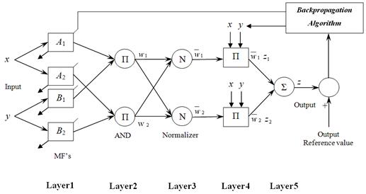
Figure 2. Corresponding ANFIS Architecture

Layer 1: Every node i in the first layer employ a node function given by:

Oi^1 = μAi(x), i = 1, 2             Oi^1 = μBi=2(y), i = 3, 4

(5)

where μ_Ai and μ_Bi can adopt any fuzzy membership function (MF).

Layer 2: Every node in this layer calculates the firing strength of a rule via multiplication:

(6)

Layer 3: The i-th node in this layer calculates the ratio of the i-th rule’s firing strength to the sum of ail rules firing strengths:

(7)

where  is referred to as the normalized firing strengths.

Layer 4: In this layer, every node i has the following function:

i = 1, 2

(8)

where  is the output of  layer 3, and { p_i, q_i, r_i} is the parameter set. The parameters in this layer are referred to as the consequent parameters.

Layer 5: The single node in this layer computes the overall output as the summation of all incoming signals, which is expressed as:

(9)

The output  in Fig. 3 can be rewritten as [9, 10]:

(10)

Adaptive Neuro-Fuzzy controller

The ANFIS controller generates change in the reference voltage V_ref, based on speed error e and derivate in the speed error de defined as:

e = ωref - ω	(11)
de = [d(ωref - ω)]/dt	(12)

where ω_ref and ω are the reference and the actual speeds, respectively.

In this study first order Sugeno type fuzzy inference was used for ANFIS and the typical fuzzy rule is:

if e is Ai and de is Bi then z = f(e, de)

(13)

where A_i and B_i are fuzzy sets in the antecedent and z = f(e, de) is a crisp function in the consequent.

The significances of ANFIS structure are:

Layer 1: Each adaptive node in this layer generates the membership grades for the input vectors A_i, i =1,…, 5. In this paper, the node function is a triangular membership function:

(14)

Layer 2: The total number of rule is 25 in this layer. Each node output represents the activation level of a rule:

,i =1, …, 5

(15)

Layer 3: Fixed node i in this layer calculate the ratio of the i-th rule's activation level to the total of all activation level:

(16)

Layer 4: Adaptive node i in this layer calculate the contribution of i-th rule towards the overall output, with the following node function:

(17)

Layer 5: The single fixed node in this layer computes the overall output as the summation of contribution from each rule:

(18)

The parameters to be trained are a_i, b_i and c_i of the premise parameters and p_i, q_i, and r_i of the consequent parameters. Training algorithm requires a training set defined between inputs and output [3]. Although, the input and output pattern set have 150 rows. Figure 3.a shows optimized membership function for e and de after trained. Figure 3.b shows Surface plot showing relationship between input and output parameters after trained. Figure 3.c shows The ANFIS model structure.

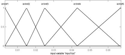
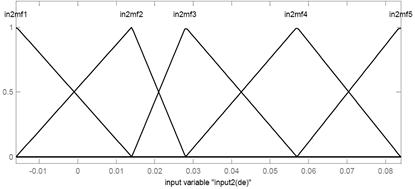
Figure 3.a. Membership functions for e and de after trained

Figure 3.b. Surface plot showing relationship between input and output parameters

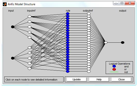
Figure 3.c. The ANFIS model structure

The number of epochs was 100 for training. The number of MFs for the input variables e and de is 5 and 5, respectively. The number of rules is then 25 (5×5 = 25). The triangular MF is used for two input variables. It is clear from (14) that the triangular MF is specified by two parameters.

Therefore, the ANFIS used here contains a total of 95 fitting parameters, of which 20 (5×2 + 5×2 = 20) are the premise parameters and 75 (3×25 = 75) are the consequent parameters.

The training and testing root mean square (RMS) errors obtained from the ANFIS are 4.7×10^-6 and 5.3×10^-6 respectively.

Particle Swarm Optimization (PSO)

PSO is a population-based optimization method first proposed by Eberhart and Colleagues [11, 12]. Some of the attractive features of PSO include the ease of implementation and the fact that no gradient information is required. It can be used to solve a wide array of different optimization problems. Like evolutionary algorithms, PSO technique conducts search using a population of particles, corresponding to individuals. Each particle represents a candidate solution to the problem at hand. In a PSO system, particles change their positions by flying around in a multidimensional search space until computational limitations are exceeded. Concept of modification of a searching point by PSO is shown in Figure 4.

(X^k: current position, X^k+ : modified position, V^k: current velocity, V^k+1: modified velocity,

V^Pbest: velocity based on Pbest, V^Gbest: velocity based on Gbest)

Figure 4. Concept of modification of a searching point by PSO

The PSO technique is an evolutionary computation technique, but it differs from other well-known evolutionary computation algorithms such as the genetic algorithms. Although a population is used for searching the search space, there are no operators inspired by the human DNA procedures applied on the population. Instead, in PSO, the population dynamics simulates a ‘bird flock’s’ behavior, where social sharing of information takes place and individuals can profit from the discoveries and previous experience of all the other companions during the search for food. Thus, each companion, called particle, in the population, which is called swarm, is assumed to ‘fly’ over the search space in order to find promising regions of the landscape. For example, in the minimization case, such regions possess lower function values than other, visited previously. In this context, each particle is treated as a point in a d-dimensional space, which adjusts its own ‘flying’ according to its flying experience as well as the flying experience of other particles (companions). In PSO, a particle is defined as a moving point in hyperspace. For each particle, at the current time step, a record is kept of the position, velocity, and the best position found in the search space so far.

The assumption is a basic concept of PSO [12]. In the PSO algorithm, instead of using evolutionary operators such as mutation and crossover, to manipulate algorithms, for a d-variable optimization problem, a flock of particles are put into the d-dimensional search space with randomly chosen velocities and positions knowing their best values so far (Pbest) and the position in the d-dimensional space. The velocity of each particle, adjusted according to its own flying experience and the other particle’s flying experience. For example, the i-th particle is represented as x_i = (x_i,1 ,x_i,2 ,…, x_i,d) in the d-dimensional space. The best previous position of the i-th particle is recorded and represented as:

Pbesti = (Pbesti,1 , Pbesti,2 ,..., Pbest i,d)

(19)

The index of best particle among all of the particles in the group is gbest_d. The velocity for particle i is represented as v_i = (v_i,1 ,v_i,2 ,…, v_i,d). The modified velocity and position of each particle can be calculated using the current velocity and the distance from Pbest_i,d to gbest_d as shown in the following formulas [13]:

	(20)
i=1,2,…,n; m=1,2,…,d	(21)

where: n = Number of particles in the group, d = dimension, t = Pointer of iterations (generations), = Velocity of particle I at iteration t, _, w = Inertia weight factor, c₁,c₂ = Acceleration constant, rand() = Random number between 0 and 1,  ₌ Current position of particle i at iterations, Pbest_i = Best previous position of the i-th particle, gbest = Best particle among all the particles in the population.

The evolution procedure of PSO Algorithms is shown in Fig. 5. Producing initial populations is the first step of PSO. The population is composed of the chromosomes that are real codes. The corresponding evaluation of a population is called the “fitness function”. It is the performance index of a population. The fitness value is bigger, and the performance is better. The fitness function is defined as follow:

(22)

where PI is the fitness value, e is the speed error and “MIN_offset” is a constant.

After the fitness function is calculated, the fitness value and the number of the generation determine whether the evolution procedure is stopped or not (Maximum iteration number reached?). In the following, calculate the Pbest of each particle and gbest of population (the best movement of all particles). The update the velocity, position, gbest and pbest of particles give a new best position (best chromosome in our proposition).

Figure 5. The evolution procedure of PSO Algorithms

Optimal ANFIS Controller Design

To design the optimal ANFIS controller, the PSO algorithms are applied to find the globally optimal parameters of the ANFIS. The structure of the ANFIS controller with PSO algorithms is shown in Figure 6.

In this paper, the chromosomes of the PSO algorithms contains two parts: the range of the membership functions (Ke and Kde) and the shape of the membership functions (e1~e5 and de1~de5). It gives the optimal output voltage, such that the steady-state error of the response is zero. The genes in the chromosomes are defined as:

[Ke, Kde, e1, e2, e3, e4, e5, de1, de2, de3, de4, de5]

(23)

Figure 7 shows the membership functions of the ANFIS controller with PSO Algorithms. Table 2 lists the parameters of PSO algorithms used in this paper.

Figure 6. ANFIS with PSO Algorithms structure

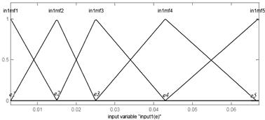
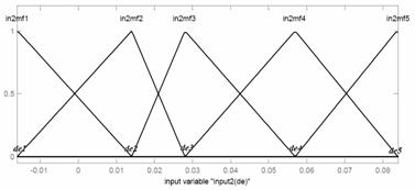
Figure 7. Membership function of ANFIS controller with PSO

Table 2. Parameters of PSO

Population Size	50
Number of Iterations	100
wmax	0.6
wmin	0.1
c1 = c2	1.5
Min-offset	200
Ke and Kde	[0.0045 ~ 0.005]
e1	[0 ~ 0.015]
e2	[0 ~ 0.025]
e3	[0.025 ~ 0.043]
e4	[0.025 ~ 0.067]
e5	[0.043 ~ 0.067]
de1	[-0.01611 ~ 0.014]
de2	[-0.01611  ~ 0.0275]
de3	[0.014 ~ 0.0565]
de4	[0.0275 ~ 0.084]
de5	[0.0565 ~ 0.084]

Computer Simulation

Three different controllers are designed for the computer simulation. First, the fuzzy logic controller is designed based on the expert experience. Second, the fuzzy logic controller is designed based on the neural networks to find the optimal range of the membership functions (ANFIS). After that, the optimal fuzzy controller (ANFIS) is designed based on the PSO to search the optimal range of the membership functions, the optimal shape of the membership functions (ANFIS with PSO).

After the primitive simulation process, the optimal values of Ke and Kde in ANFIS are calculated as 0.005 and 0.005, respectively. The best chromosomes in ANFIS with PSO are pursued as:

[0.004751, 0.004974, 0.006037, 0.012420, 0.031521, 0.050601, 0.065930, -0.00353, 0.017701, 0.032000, 0.052880, 0.078040]

(24)

The optimal membership functions ANFIS with PSO are shown in Figure 8.

Let the command signal be a step for the speed of the DC motor at 127.93 Rad/Sec. The simulation results are obtained for 0.01 second range time.

The speed response of FLC (Fuzzy Logic Controller) is shown in Fig 9. The speed response of FLC using neural networks (ANFIS) is shown in Fig 10. The speed response of the optimal ANFIS controller using PSO is shown in Fig 11.

The performances of three controllers are listed in Table 3.

According to our MATLAB model simulation, we illustrate that the steady state error equal zero in one case: ANFIS controller with PSO (ANFIS-Swarm); the overtaking value is zero in the three cases that means the FLC used is robust. The rising time of DC motor speed step is less important in FLC using neural networks (ANFIS) compared with FLC alone and it’s have the minimal value in The ANFIS controller with PSO (ANFIS-Swarm).

In the present work, the intelligent controller based on ANFIS-Swarm optimization give a good agreement with the step reference speed. In the Adaptive Neuro-Fuzzy (ANFIS)  DC motor control, the optimization of membership functions became very necessary, it’s important shown in the minimal rising time of speed response, so the membership functions are adjusted in optimal values to give a steady state error speed value equal zero. The computer MATLAB simulation demonstrate that the ANFIS controller associated to the Swarm intelligence approach became very strong, it gives a very good results and possesses good robustness.

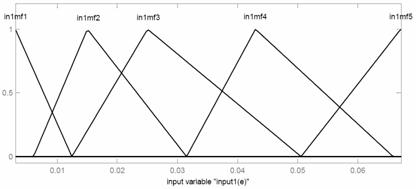
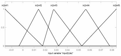
Figure 8. The optimal membership functions ANFIS with PSO

Figure 9. The speed response of Fuzzy Logic Controller

Figure 10. The speed response of FLC using neural networks (ANFIS)

Table 3. Performances of three controllers

Results	Fuzzy Logic Controller(FLC)	FLC using neural networks (ANFIS)	ANFIS controller with PSO (ANFIS-Swarm)
Rising time [Sec]	0.00385	0.00301	0.00285
Overtaking [%]	0	0	0
Steady state error[%]	9×10^-4	3.2×10^-4	0

Conclusions

In this paper, the optimal ANFIS controller is designed using Particle Swarm Optimization algorithms. The speed of a DC Motor drive is controlled by means of three different controllers. According to the results of the computer simulation, the Adaptive Neuro-Fuzzy (ANFIS) controller efficiently is better than the traditional FLC. The ANFIS-Swarm is the best controller which presented satisfactory performances and possesses good robustness (no overshoot, minimal rise time, Steady state error = 0). The major drawback of the fuzzy controller presents an insufficient analytical technique design (choice of the rules, the membership functions and the scaling factors). That we chose with the use of the Neural Networks and Particle Swarm Optimization for the optimization of this controller in order to control DC motor speed. Finally, the proposed controller (ANFIS-Swarm Controller) gives a very good results and possesses good robustness.

References

1. Hénao H., Capolino G. A.  Méthodologie et application du diagnostic pour les systèmes électriques. Article invité dans Revue de l'Electricité et de l'Electronique (REE), (Text in French) 2002, 6, p. 79-86.

2. Raghavan S. Digital control for speed and position of a DC motor. MS Thesis, Texas A&M University, Kingsville, 2005.

3. Jang J. S. R. Adaptive network based fuzzy inference systems. IEEE Transactions on systems man and cybernetics 1993, p. 665-685.

4. Shi Y., Eberhart R. A modified particle swarm optimizer. Proc. 1998 Int. Conf. on Evolutionary Computation–The IEEE World Congress on Computational Intelligence, Anchorage 1998, p. 69-73.

5. Clerc M., Kennedy J.  The particle swarm-explosion, stability, and convergence in a multidimensional complex space. IEEE Trans. Evolutionary Computation 2002, 6, p. 58-73.

6. Halila A.  Étude des machines à courant continu. MS Thesis, University of LAVAL, (Text in French), May 2001.

7. Capolino G. A., Cirrincione G., Cirrincione M., Henao H., Grisel R. Digital signal processing for electrical machines. Invited paper, Proceedings of ACEMP'01 (Aegan International Conference on Electrical Machines and Power Electronics), Kusadasi (Turkey), 2001, pP. 211-219.

8. Lin C. T., Lee C. S. G. Neural fuzzy systems: A neuro-fuzzy synergism to intelligent systems. Upper Saddle River, Prentice-Hall, 1996.

9. Constantin V. A. Fuzzy logic and neuro-fuzzy applications explained. Englewood Cliffs, Prentice-Hall, 1995.

10. Kim J., Kasabov N. Hy FIS, Adaptive neuro-fuzzy inference systems and their application to nonlinear dynamical systems. Neural Networks, 1999.

11. Kennedy J., Eberhart R.  Particle swarm optimization. Proc. IEEE Int. Conf. on Neural Network 1995, 4, p. 1942-1948.

12. Yoshida H., Kawata K., Fukuyama Y., Takayama S., Nakanishi Y.. A particle swarm optimization for reactive power and voltage control considering voltage security assessment.  IEEE Trans. on Power Systems 2000, 15(4), p. 1232-1239.

13. Gaing Z. L. A particle swarm optimization approach for optimum design of PID controller in AVR system. IEEE Trans. Energy Conversion 2004, 19, p. 384-391.