A New Approach for Control of IPFC for Power Flow Management
E-mail(s):
asad@iust.ac.ir, kazemi@iust.ac.ir
(* Corresponding author: Phone: +98 21 77240492
Fax: +98 21 77240490)
Abstract
The Interline Power Flow Controller (IPFC) is one of the Voltage Source Converter (VSC) based facts controllers which can effectively manage the power flow via multi-line transmission system. In this paper a new method for control of IPFC, with the aim of managing the power flow in transmission lines is presented. Simplicity and fast system response are two characteristics of this method. An IPFC with the presented control method is simulated. The results of this simulation demonstrate the success of the method.
Keywords
FACTS, Interline Power Flow Controller (IPFC), Power Flow Control, Voltage Source Converter (VSC).
Introduction
The FACTS controllers which have been introduced during the last two decades, are able to improve the transmission Systems. Some of the advantages of the utilization of these devices in transmission systems are increasing in maximum transmissible power in transmission lines, improving in the stability of transmission systems especially when a fault occurs, and decreasing in line losses. These advantages are not achievable with traditional mechanical switches based approaches because of lack of continuous control and the necessity of large stability margin [1] with them.
IPFC has different applications. Equalizing active and reactive power flows through compensated transmission lines, transmitting power from over-loaded lines to other lines, compensation of resistive voltage drops through lines and improving the performance of the compensated system when dynamic disturbances occur, are some applications of IPFC [1]. In general, an IPFC consists of N (the number of compensated lines by IPFC) voltage source inverters which have common dc link. In other words, it can be said that IPFC consists of a number of SSSC with common dc link [1].
In 2002, a research group presented two general methods for control of IPFC [1]. Unfortunately one of the characteristic of these two methods was heavy calculations. In the same year, another control method, based on fuzzy logic, was implemented on IPFC by another group [2]. The specialty of the presented method by this group, was concerning of the nonlinearity characteristic and the effects of the inverters of IPFC on each other. The result of another research on control of IPFC, was a complex control method using adaptive control, genetic algorithm and neural network simultaneously [3].
n This paper, a new control method with two specialty of simplicity and the lack of necessity of heavy calculations, is presented for IPFC. The good performance of the proposed control method is also demonstrated by the simulation results at end of this paper.
Structure and Behavior of IPFC
IPFC consists of N voltage source inverters (VSI) by which the compensation of N lines is done. These inverters have a common dc link through which they are connected to each other and exchange active power with each other. It is obvious that the algebric sum of the exchanging powers through inverters and lines should be zero. Otherwise, dc link voltage (which consists of a capacitor) and, in result, the output voltages of the inverters will be changed.
In practice, there is an N-line transmission system equipped with IPFC, then N-1 lines are assumed as primary lines and the Nth line left is assumed as auxiliary line [1]. The auxiliary line provides the active power needed by the N-1 primary lines [1]. This fact should be considered in designing the control system of the inverter of the auxiliary line. For simplicity of study for behavior of IPFC, it is assumed that the controlled lines by the IPFC, are two similar lines (V1s = V1r = V2s = V2r = V, δ1 = δ2 = δ, L1 = L2 = L, R1 = R2 = R) (Figure 1).

Figure 1. The interline power flow controller compensating two lines
Figure 2 Shows the equivalent circuit of IPFC [4,5]. In this figure the dc relationship of the two inverters through which active power is exchanged, is represented by a bi-directional flash [1]. In accordance with Fig. 1, the active and reactive power flow in both of the lines can be calculated by the following relationships:
|
|
(1) |

where i is the line index, V1 equals to Vr – Vs, φ = cos-1(R/√(R2 + (Lω)2)) and θipq is the phase difference between Vipq and V1 [5].
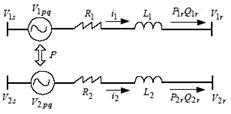
Figure 2. Equivalent circuit of IPFC shown in figure 1
Figure 3 depicts the vector diagram of voltages and currents of the two controlled lines by IPFC. As can be seen Vr is considered as the reference vector. The circle shown in the figure determines the limits of the output voltages of the two inverter. The radius of this circle is equal to the maximum amplitude of the output voltages of the two inverters which is a function of common dc link voltage. The lines in the circle which are parallel with vector V1 (Vr - Vs) are called "voltage compensation lines". Whenever the tip of output voltage vector of one of the inverters remains on a voltage compensation line, the active power exchange between the inverter and the corresponding line will remain constant [6].

Figure 3. Vector diagram of currents and voltages of the lines and IPFC
The voltage compensation line which crosses the center of the circle and has the same direction as V1, is the locus of the output voltages which don't exchange energy with transmission lines. In this paper, this voltage compensation line is called “exchange-free line”. In fact, when the tip of output voltage vectors is on exchange-free line, the two inverters act as two independent SSSC.
The voltage compensation lines which are in the right side of exchange-free line, are corresponding to the output voltages which cause injection of active power to transmission line, and the voltage compensation lines which is in the left side of exchange-free line, are corresponding to the output voltages which cause absorption of active power from transmission line. So to make the algebric sum of the exchanging power of the two inverters with the lines is zero, the tip of the output voltage vectors of the two inverters should be on the two voltage compensation lines which are at different sides of exchange-free line and have the same distance to the center of the circle. This is the only limitation that should be considered for the voltages of the two inverters. Now by moving the tip of the output voltage vectors on the two voltage compensation lines, the active and reactive power flows of the two transmission lines can be controlled and in this way the two transmission lines shown in Fig. 1 will be compensated as desired. Of course It should be noted that the compensation is restricted because of the limitation mentioned above [4,5]. Fig. 4 illustrates this fact by showing the maximum possible amount of the variations of Pr and Qr when the tip of voltage vector of one of the two inverters moves on its corresponding voltage compensation line.

Figure 4. The compensation area of IPFC when its operating point is moving on the voltage compensation line 2
Principles of Control of IPFC
Assume that in Fig. 1, line1 is the primary line and line2 is the auxiliary line. For control of IPFC firstly the operating point of the primary inverter, according to the desired type of compensation for the primary line, is determined independently and then the operating point of the inverter of the auxiliary line, considering the only limitation discussed before and the desired type of compensation for the auxiliary line is determined. In other words, the tip of output voltage vector of inverter1 can freely move in the circle shown in Figure 3, but the tip of output voltage vector of inverter2 can only move on the voltage compensation line which is located in the opposite side of the voltage compensation line corresponding to output voltage of inverter1. So there are two degrees of freedom for the compensation of line1 but there is only one degree of freedom for the compensation of line2. In other words, comparing to line1, there is some more limitation for compensation of line2. To explain more, the reason is that it is the duty of inverter2 to keep common dc link voltage constant. Therefore, as said before, there is no need to limit the operating point of inverter1 to prevent the variations of common dc link voltage. So in design of the control system of this inverter of IPFC, the inverter can be assumed as a voltage source inverter equipped with an energy storage system, for example a battery. In this condition, it is obvious that in design procedure of the control system of inverter1, there is no concern about the variation of common dc link voltage.
Despite the difference between inverter1 and inverter2, with some modifications, the control system of inverter1 can also be used for inverter2. To do this, at first the control of one of the two characteristics of the line which are controlled by the control system of inverter1, should be ignored. In fact, regardless of the control method chosen for IPFC, this ignorance always should be done. The reason is the mentioned limitation in the compensation of line2. For example if the aim of the control system of inverter1 is control of both of the transmitted active and reactive power, then when it is wanted to use this control system for inverter2, the feedback loop of one of the transmitted active or reactive power should be omitted. In this way, only one of the transmitted active or reactive power is controlled and the value of the other characteristic of line2 whose feedback loop has been omitted will be determine by the control system of the dc link voltage. In fact, the value of the characteristic whose feedback loop has been omitted, is determined in a way that a proper value of active power will be exchanged between intverter2 and the corresponding line to make common dc link voltage remain constant.
A New Method for Control of IPFC
As it is known, the main aim of utilizing FACTS controllers is the control of power flow in transmission lines [8]. So the aim of the control system of IPFC presented in this paper is control of power flow too.
If d and q axis's are defined as shown in Fig. 5 and the ohmic resistances of transmission lines are ignored, relationships (1) can be writhen as:
|
|
(2) |
where V1q, V1d, Vr
and |Z| all are constant. The recent relationships imply two
notes. First Pir and Qir can be controlled
by control of ![]() and
and ![]() respectively.
Second the control of Pir and Qir are
completely independent, so that by changing the value of one of them, the other
one won't change [5]. Considering these two notes, a control circuit whose
block diagram is shown in Fig. 6, is presented to control the active and
reactive power flow in line1. As can be seen in Fig. 6, any difference between
the measured and reference values of active or reactive power flow cause proper
changes (
respectively.
Second the control of Pir and Qir are
completely independent, so that by changing the value of one of them, the other
one won't change [5]. Considering these two notes, a control circuit whose
block diagram is shown in Fig. 6, is presented to control the active and
reactive power flow in line1. As can be seen in Fig. 6, any difference between
the measured and reference values of active or reactive power flow cause proper
changes (![]() or
or ![]() ) in corresponding
voltage components (
) in corresponding
voltage components (![]() or
or ![]() ) with the aid of a
proper PI controller, to make the measured and reference values of the active
and reactive power flows equal.
) with the aid of a
proper PI controller, to make the measured and reference values of the active
and reactive power flows equal.
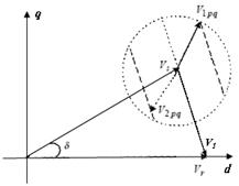
Figure 5. The definition of d and q axis’s
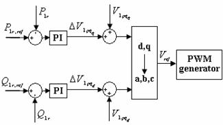
Figure 6. The block diagram of control circuit of inverter 1
The presented
control circuit of inverter1 can be used to control inverter2 too. But to do
this, as described before, the control of one of the active or reactive power
flow (in this paper, the control of active power flow was ignored) should be
ignored by omission of its feedback loop in the circuit (Figure 7). To control
the dc link voltage (or to compensate the active power exchanged with line1 by
inverter1), in the presented control circuit of Figure 7 proper voltages are
added to the two components of the output voltage of inverter2 which are
determined before according to the reference reactive power flow of line2. The
phase of the added voltage, whose duty is exchanging a proper amount of active
power with line2 to control dc link voltage, is set equal to the phase of the
current of line2 (i2) by the phase lock loop and its
amplitude is set proportional to the algebric sum of the active powers
exchanged with the lines by inverters 1 and 2 (![]() ). In this way, having
equal phase with the current of line2, this voltage only influences on the
amount of the active power exchanged between inveter2 and line2. Also, this
voltage whose amplitude is set as explained above; make the difference between
the active powers exchanged with the lines by the inverters, become equal to
zero. With this strategy, the active power provided for a line by the dc link,
will be equal to the active power injected to the dc link by the other line.
Therefore the dc link voltage will remain constant. The block diagram of the
applied control circuit for inverter2 is shown in Fig. 7. As seen, the control
of the active power flow of line2 has been ignored.
). In this way, having
equal phase with the current of line2, this voltage only influences on the
amount of the active power exchanged between inveter2 and line2. Also, this
voltage whose amplitude is set as explained above; make the difference between
the active powers exchanged with the lines by the inverters, become equal to
zero. With this strategy, the active power provided for a line by the dc link,
will be equal to the active power injected to the dc link by the other line.
Therefore the dc link voltage will remain constant. The block diagram of the
applied control circuit for inverter2 is shown in Fig. 7. As seen, the control
of the active power flow of line2 has been ignored.
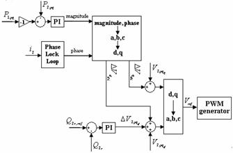
Figure 7. The block diagram of control circuit of inverter 2
Simulation Results
The presented
method for control of IPFC, was simulated for two
similar lines (Figure 1). In the simulation, the resistances of the lines were
ignored, the reactance of each line (X) was 0.5 p.u.,
the voltages of the beginning and the end of the lines (Vs and Vr)
were 1 p.u. and the phase difference between the voltages of the beginning and
the end of the lines ![]() was -30 degree. Also, the
parameters of the control circuits shown in Figure 6 and Figure 7, have been considered as described in Table 1.
was -30 degree. Also, the
parameters of the control circuits shown in Figure 6 and Figure 7, have been considered as described in Table 1.
Table 1. The Parameters of the Control Circuits
|
KI |
KP |
Control Loop |
Control Circuit |
|
0.1 |
0.008 |
Active Power |
Line 1 |
|
0.1 |
0.3 |
Reactive Power |
|
|
--- |
--- |
Active Power |
Line 2 |
|
0.1 |
0.3 |
Reactive Power |
|
|
8 |
0.1 |
dc Link |
In the simulation, at first the parallel lines are in the steady state mode and without IPFC (P1r = P2r = 1 p.u., Q1r = Q2r = -0.268 p.u.). Then at t = 0.1 s IPFC with the reference values of P1r = 1 p.u., Q1r = 0 p.u. and Q2r = -0.5 p.u., which are the same as [6], starts operating. Figure 8 shows active and reactive power flows of transmission lines during the simulation. As seen in this figure, the active and the reactive power flows of line 1 are controlled as desired. Also the IPFC makes reactive power flow of line2 becomes -0.5 p.u. with a good approximation. The reason of the small difference between the measured and the reference values of reactive power flow in line2 is the second duty of inverter2 which is the control of the common dc link voltage. In other words, although the value of active power flow of line2 is set by the control circuit in a way that the dc link voltage remains constant, but the control of the dc link voltage has a little influence on control of reactive power flow too.
|
|
|
|
(a) |
(b) |

Figure 8. Active and reactive power flow in p.u.: (a) in line 1; (b) in line 2
|
|
|
|
(a) |
(b) |


Figure 9. Exchanged active power (p.u.) with the lines: (a) inverter 1 (P1pq); (b) inverter 2 (P2pq)
To illustrate the success of the presented control system in keeping the dc link voltage constant, the exchanged active powers with the two lines by the inverters were depicted in Fig. 9. It can be seen in this figure that the exchanged active powers rapidly get equal in amplitude but different in sign, as it is necessary for control of the dc link voltage.
As it is known, IPFC controls power flow by the injection of proper series voltages in transmission lines with the aid of its inverters. Figure 10 shows the currents and output voltages of invertors 1 and 2 in the simulation.
It can be seen in Figure 6 and Figure 7 that the reference voltage (Vref( for each of the inverters of the IPFC is constructed by q and d components which are properly determined by the control circuits. In Figure 11 the amplitude of the q and d components for both of the inverters are shown. Simulation results show that after start of operation of IPFC at t = 0.1 s, the system is in the transient state during the first 0.09 s and then it is in the steady state. The short time duration of the transient state, illustrates the high speed of the presented control method.
|
|
|
|
(a) |
(b) |
Figure 10. Voltage and current of inverters (p.u): (a) in line 1; (b) in line 2
|
|
|
|
(a) |
(b) |
Figure. 11. q and d components of voltage (p.u.): (a) inverter 1; (b) inverter 2
Conclusions
In this paper, according to the structure and behavior of IPFC and also the principals of its control, a new method for control of IPFC, with the aim of managing power flow in transmission lines, was presented. Some of the advantages of this method are fast system response, few calculations, so that the high speed processors are not required for this method, and simplicity. These advantages make this method an interesting practicable control method for IPFC. In this method, because of the well designed control circuit, all the required calculations are done automatically with the aid of proper feedbacks. To validate the control method, results of the simulation of an IPFC with the control method were presented. These results proved the success of this method.
References
1. Chen J., Lie T.T., Vilathgamuwa D. M., Basic Control of Interline Power Flow Controller, Power Engineering Society Winter Meeting, IEEE 2002, 1, p. 521- 525.
2. Menniti D., Pinnarelli A., Sorrentino N., A fuzzy logic controller for interline power flow controller model implemented by ATP-EMTP, Proceedings. Power System Technology, 2002, 3, p. 1898-1903.
3.
Mishra S., Dash P.K., Hota P.K., Tripathy M., Genetically optimized
neuro-fuzzy IPFC for damping modal oscillations of power system,
4.
Gyugyi L., Sen K. K., Schauder C.D., The
Interline Power Flow Controller Concept: A New Approach to Power Flow
Management in Transmission Systems,
5. Zhang L., Crow M.L., Yang Z., Chen S., The Steady State Characteristics of an SSSC Integrated With Energy Storage, Power Engineering Society Winter Meeting, IEEE, 2001, 3, p. 1311-1316.
6.
Gyugyi L., Sen K.K., Schauder C.D., The
Interline Power Flow Controller Concept: A New Approach to Power Flow
Management in Transmission Systems,
7. Ghosh A., Shukla A., Joshi A., Flying Capacitor Multilevel Inverter and its Applications in Series Compensation of Transmission Lines, Proceedings. IEEE/PES General Meeting, 2004, p. 1516-1521.
8. Urbanek J., Piwko R.J., Larsen E.V., Damsky B.L., Furumasu B.C., Mittlestadt W., Eden J.D., Thyristor controlled series compensation prototype installation at the SLATT 500 kV substation, IEEE Transactions on Power Delivery, 1993, 8(3), p. 1460-1469.