Artificial Neural Network Application for Power Transfer Capability and Voltage Calculations in Multi-Area Power System

Palukuru NAGENDRA^*, Sunita Halder nee DEY and Tanaya DUTTA

Department of Electrical Engineering, Jadavpur University, Kolkata-700032, West Bengal, India

E-mail: indrapn@gmail.com; sunitaju@yahoo.com; tanayadatta21@yahoo.co.in

(^* Corresponding author: Phone: 09804353148, Fax: 03324146184)

Abstract

In this study, the use of artificial neural network (ANN) based model, multi-layer perceptron (MLP) network, to compute the transfer capabilities in a multi-area power system was explored. The input for the ANN is load status and the outputs are the transfer capability among the system areas, voltage magnitudes and voltage angles at concerned buses of the areas under consideration. The repeated power flow (RPF) method is used in this paper for calculating the power transfer capability, voltage magnitudes and voltage angles necessary for the generation of input-output patterns for training the proposed MLP neural network. Preliminary investigations on a three area 30-bus system reveal that the proposed model is computationally faster than the conventional method.

Keywords

Artificial neural networks; Multi-layer perceptron; Levenberg-Marquardt algorithm; Power transfer capability; Repeated power flow.

Major Symbols

Pr = real power interchange between areas	k = bus not in receiving area
Pkm = tie line real power flow (from bus k in sending area to bus m in receiving area)	m = bus in receiving area
Yij, θij = magnitude and angle of ij^th element of admittance of matrix Y	R = set of buses in receiving area
Vi, δi = magnitude and angle of voltage at i^thbus	n = set of all the buses
Pg, Qg = real and reactive power outputs of generator	Pi, Qi = net real and reactive powers at bus i
Sij = apparent power flow through transmission line between bus i and bus j

Introduction

Modern power systems are operating closer to their operating limits due to economic reasons and operational factors arising out of deregulation [1,2] and open market of electricity. Under such stressed conditions, the transfer capability becomes a major concern in system operation and planning [3, 4]. Power system transfer capability indicates how much inter area power transfers can be increased without compromising system security. Transfer capability computations are performed by the system operators to know the ability of the system to transfer power among areas within the system, and also by the system planners to indicate system’s strength.

As the operating conditions of an interconnected power network vary continuously in real time, the power transfer capability of the network will also vary from instant to instant. For this reason, transfer capability and voltage calculations may need to be updated periodically for application in the operation of the network. In addition, depending on actual network conditions, transfer capabilities can often be different from those determined in the off-line studies. The most commonly used algorithms for computing power transfer capability are continuation power flow (CPF), optimal power flow (OPF) and repeated power flow methods [5, 6].

To give fast solutions to complex problems, some of which were hitherto revealed intractable by standard computing devices, artificial neural networks have recently been applied in different fields of research [7]. Many interesting ANN applications have been reported also in power system areas, where they are widely used in load forecasting, unit commitment, economic dispatch, security assessment, fault diagnosis and alarm processing [8]. Neural computing has attractive features, such as its ability to tackle new problems which are hard to define or difficult to solve analytically, its robustness in dealing with incomplete or fuzzy data, its processing speed, its flexibility and ease of maintenance.

In this paper, standard neural network architecture, multi-layer perceptron model for the computation of power transfer capabilities and voltages of multi-area power system has been proposed. The repeated power flow method, which repeatedly solves power flow equations at a succession of points along the specified load/generation increment, is used in this work for transfer capability and voltage calculations necessary for the generation of input-output patterns for training the proposed artificial neural network. The effectiveness of the ANN based approach is demonstrated on a three area 30-bus system for different loading patterns.

Conventional Repeated Power Flow Method

Referring to Fig.1, a simple interconnected power system is divided into three kinds of areas: receiving area, sending area and external areas. “Area” may be an individual electric system, power pool, control area, sub-regions, etc., which consist of a set of buses. The power transfer between two areas is the sum of the real powers flowing on all the lines which directly connect one area to the other.

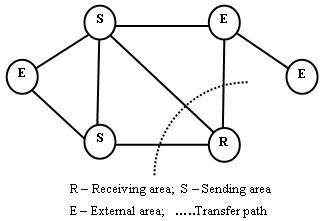
Figure 1. A Simple Interconnected Power System

The objective is to determine the maximum real power transfers from sending areas to receiving areas through the transfer path. In the mathematical formulation of the transfer capability computations problem, the following assumptions are made:

§ The base case power flow of the system is feasible and corresponds to a stable operating point.

§ The load and generation patterns vary very slowly so that the system transient stability is not jeopardized.

§ The system has sufficient damping to keep within steady state stability limit.

§ Bus voltage limits are reached before the system reaches the nose point and loses voltage stability.

The objective function to be optimized is

(1)

Subject to the power flow constraints given by

                                                                        (2)

                                                                      (3)

and the operational constraints

                                                                                               (4)

                                                                                             (5)

(6)

(7)

The control variables in this formulation are generator real and reactive power outputs, generator voltage settings, phase shifter angles, transformer taps and switching capacitors or reactors. The dependent variables are active and reactive power injections at slack bus, reactive power injection and bus voltage angle at generator buses.

The repeated power flow algorithm for the calculation of transfer capability is as follows.

1. Establish and solve the power flow problem for a base case.

2. Select a transfer case and solve for it.

3. Step increase in transfer power and solve for power flow problem.

4. Check for security limit violations of power flow through tie lines. If no violation, go back to step 3.

5. If there is any violation, decrease step size with minimum possible amount to eliminate them. This is the power transfer capability for the selected transfer case.

Multi-layer Perceptron Neural Network Model

Artificial neural networks were designed to mimic the characteristics of biological neurons in the human brain and nervous system. The network ‘learns’ by adjusting interconnections between layers. When the network is adequately trained, it is able to generalize relevant output for a set of input data. Learning typically occurs by example through training, where training algorithm iteratively adjust the connection weights (synapses).

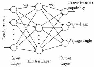
Figure 2. Proposed MLP Structure with one Hidden Layer

An MLP network consists of three layers: an input layer, an output layer, and one or more hidden layers [7]. Fig.2 illustrates a three-layered multi-layer perceptron network (MLPN). Each layer is composed of a predefined number of neurons. The neurons in the input layer only act as buffers for distributing the input signals x_i to neurons in the hidden layer. Each neuron j in the hidden layer sums up its input signals x after weighting them with the signals of the respective connections w_ji from the input layer, and computes its output y_j as a function f of the sum:

                                                                                                     (8)

where f is the activation function that is necessary to transform the weighted sum of all signals impinging onto a neuron. f is usually a sigmoidal or hyperbolic tangent function. The outputs of neurons in the output layer are computed similarly. Training a network consists of adjusting its weights using a training algorithm. In this paper the Levenberg-Marquardt (LM) algorithm [9] is used for training the MLP network. The LM algorithm is basically a Hessian based algorithm for nonlinear least square optimization. For neural network training the objective function is the error function of the type

                                                                                                (9)

where  y_k  is the actual output for the k^th pattern and t_k  is the desired output. p is the total number of training patterns.

The steps involved in training a neural network using LM algorithm are as follows:

1. Present all inputs to the network and compute the corresponding network outputs and errors. Compute the mean square error over all inputs as in (9).
2. Compute the Jacobian matrix, J(w) where w represents the weights and biases of the network.
3. Solve the Levenberg-Marquardt weight update equation to obtain Dw.
4. Recompute the error using w+Dw. If this new error is smaller than that computed in step 1, then reduce the training parameter m by m^-, let w= w+ Dw, and go back the step1. If the error is not reduced, then increase m by m⁺, and go back step 3.
5. The algorithm is assumed to have converged when the norm of the gradient is less than some predetermined value, or when the error has been reduced to some error goal.

The weights are updated according to the following formula:

                                                                                  (10)

with                                                                    (11)

where E is a vector of size p calculated as

                                                                          (12)

where J^T(w)J(w) is referred as the Hessian matrix. is the identity matrix, m is the learning parameter.

Test System and Simulation Results

The proposed MLPN model is applied to a three area 30-bus system, the single line diagram of which is given in Fig. 3. The system data is given in appendix. The system is arbitrarily divided into three areas with 2 generators in each area. The power transfer capabilities between area 2 and area 3 are investigated for different loading conditions obtained by varying the active and reactive power loads in the system. The loads are varied with uniform power factor in such a way that the new load condition remains with in a range of 80 – 120% of the base operating condition of the system under consideration. In this study, using the RPF-based algorithm, the transfer capability from area 2 to area 3, bus voltage magnitudes and voltage angles in these areas are computed for different loading conditions. This data is then used to train the ANN to provide real time evaluation of transfer capability, voltage magnitudes and voltage angles. Once the ANN is trained, the ANN ‘learns’ the implicit correlation between the loading patterns and the transfer capability patterns. Next, the new loading patterns (which have not been used to train the ANN) would be fed to the network and the network would provide the optimal   power   transfer   capability, voltage magnitude and voltage angles at its output. The performance of the proposed MLPN method is presented in terms of relative error (ε), which is defined as

                                                                                                (13)

where t_i is the exact value from repeated power flow solutions and o_i is the output of ANN.

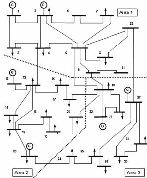
Figure 3. Three area 30-bus system

Table I shows the comparison of transfer capabilities from area 2 to area 3 obtained with proposed MLPN model against those obtained with the RPF method for different load operating conditions. The bus voltage magnitudes and voltage angles, calculated by the two methods for the power transfer capability case of area 2 to area 3 for 107.5% base operating condition are given in Table II. Fig. 5 and Fig. 6 show graphically the comparison of bus voltage magnitudes and voltage angles respectively calculated by the two methods for the transfer capability case of area 2 to area 3 for 112.5% base operating condition. From the simulation results, it can be seen that the proposed MLPN model is giving the results practically as accurate as that of conventional method. Further, it was observed that the proposed network with 16 inputs, 3 outputs and 9 neurons in the hidden layer takes only 0.94 second for an error goal of 1e^-4, while the conventional method takes 2.81 seconds for the same computation.

Table 1. Transfer Capability from Area 2 to Area 3: Comparison of RPF and MLPN methods

Load Condition (%)	Transfer capability, MW		Relative error (%)
	RPF method	MLPN method
92.5 97.5 102.5 107.5 112.5 117.5	26.4708 24.5007 23.1758 21.5064 19.8220 18.1225	26.4746 24.5113 23.1868 21.5106 19.8236 18.1270	0.0143 0.0432 0.0474 0.0195 0.0080 0.0248

Table 2. Voltage Magnitudes and Voltage Angles of Area 2 and Area 3 (107.5% Load Condition)

Bus no.	Bus Voltage magnitude, p.u.		Bus Voltage angle, deg.
	RPF method	MLPN method	RPF method	MLPN method
10 12 13 14 15 16 17 18 19 20 21 22 23 24 25 26 27 29 30	0.9777 0.9756 1.0000 0.9592 0.9661 0.9632 0.9657 0.9440 0.9400 0.9465 0.9916 1.0000 1.0000 0.9870 0.9891 0.9697 1.0000 0.9780 0.9653	0.9776 0.9756 1.0000 0.9592 0.9661 0.9630 0.9655 0.9440 0.9400 0.9465 0.9917 1.0000 1.0000 0.9870 0.9891 0.9697 1.0000 0.9780 0.9653	-4.7099 -3.5361 -0.4925 -4.5277 -4.5333 -4.5184 -4.9607 -5.7293 -6.1094 -5.8632 -4.7017 -4.5653 -3.8722 -3.9179 -1.8301 -2.3150 -0.2429 -1.6428 -2.6284	-4.7077 -3.5341 -0.4905 -4.5257 -4.5312 -4.5163 -4.9584 -5.7271 -6.1071 -5.8610 -4.6993 -4.5628 -3.8699 -3.9154 -1.8272 -2.3120 -0.2398 -1.6321 -2.6248

Conclusions

In this paper, an artificial neural network model, multi-layer perceptron network has been developed for the computation of the power transfer capability among various areas and voltage magnitudes and voltage angles of the concerned buses of those areas in an interconnected system, accurately and rapidly for any loading conditions. Repeated power flow based transfer capability computation algorithm is utilized in generating the input-output patterns required for training the proposed ANN model. The preliminary investigations on a multi-area system indicate that the proposed model is computationally faster than the conventional RPF method and is useful for online applications.

References

1. William W.H., John F.K., Electricity market restructuring: Reforms after reforms, 20^th Annual Conference Center for Research in Regulated Industries, May 2001.

2. Mala D., Pricing of system security in deregulated environment, Int. J Recent Trends in Engineering, 2009, 1(4), p. 49-51.

3. Ian D. et al., Electric power transfer capability: Concepts, applications, sensitivity and uncertainty, PSERC publication, 2001, p. 1-34.

4. Yan O., Singh C., Assessment of available transfer capability and margins, IEEE Trans. Power Systems, 2002, 17(2), p. 463-468.

5. Ajjarapu V., Chrity C., The continuation power flow: A tool for steady state voltage stability analysis, IEEE Trans. Power Systems, 1992, 17(1), p. 416-423.

6. Chakrabarti A., Sunita Halder, Power system analysis: operation and control, New Delhi, India, Prentice Hall of India (pvt) Ltd., 2^nd edition, 2008.

7. Haykin S., Neural Networks – A comprehensive foundation, Prentice Hall Ltd, New York, 1999.

8. Vidya Sagar S.V., Rao N.D., Artificial neural networks and their applications to power systems-a bibliographical survey, Electric Power Systems Research, 1993, 28, p. 67-69.

9. Deepak M., Abhishek Yadav, Sudipta R., Prem K. K., Levenberg-Marquardt learning algorithm for Integrate-and-Fire neuron model, Neural Information Processing-Letters & Reviews, 2005, 9(2), 41-51.

Appendix

30-bus test system data is given below.

Table A1. Bus Data

SB	EB	R (p.u)	x (p.u)	b (p.u)	Line limit (MW)
1	2	0.02	0.06	0.03	130
1	3	0.05	0.19	0.02	130
2	4	0.06	0.17	0.02	65
3	4	0.01	0.04	0.00	130
2	5	0.05	0.20	0.02	130
2	6	0.06	0.18	0.02	65
4	6	0.01	0.04	0.00	90
5	7	0.05	0.12	0.01	70
6	7	0.03	0.08	0.01	130
6	8	0.01	0.04	0.00	32
6	9	0.00	0.21	0.00	65
6	10	0.00	0.56	0.00	32
9	11	0.00	0.21	0.00	65
9	10	0.00	0.11	0.00	65
4	12	0.00	0.26	0.00	65
12	13	0.00	0.14	0.00	65
12	14	0.12	0.26	0.00	32
12	15	0.07	0.13	0.00	32
12	16	0.09	0.20	0.00	32
14	15	0.22	0.20	0.00	16
16	17	0.08	0.19	0.00	16
15	18	0.11	0.22	0.00	16
18	19	0.06	0.13	0.00	16
19	20	0.03	0.07	0.00	32
10	20	0.09	0.21	0.00	32
10	17	0.03	0.08	0.00	32
10	21	0.03	0.07	0.00	32
10	22	0.07	0.15	0.00	32
21	22	0.01	0.02	0.00	32
15	23	0.10	0.20	0.00	16

Table A2. Load Data

Bus No.	Pd (MW)	Qd (MVAR)
2	21.7	12.7
3	2.4	1.2
4	7.6	1.6
7	22.8	10.9
8	30.0	30.0
10	5.8	2.0
12	11.2	7.5
14	6.2	1.6
15	8.2	2.5
16	3.5	1.8
17	9.0	5.8
18	3.2	0.9
19	9.5	3.4
20	2.2	0.7
21	17.5	11.2
23	3.2	1.6
24	8.7	6.7
26	3.5	2.3
29	2.4	0.9
30	10.6	1.9

Table A3. Generator Data

Bus No.	Pg (MW)	Qg (MVAR)	Qmax (MVAR)	Qmin (MVAR)	Vg (p.u)	Pmax (MW)	Pmin (MW)
1	23.54	0.00	150.0	-20.0	1	80	0
2	60.97	0.00	60.0	-20.0	1	80	0
22	21.59	0.00	62.5	-15.0	1	50	0
27	26.91	0.00	48.7	-15.0	1	55	0
23	19.20	0.00	40.0	-10.0	1	30	0
13	37.00	0.00	44.7	-15.0	1	40	0