Development of Graphical User Interface for Finite Element Analysis of Static Loading of a Column using MATLAB
Moses Omolayo PETINRIN
Prototype Engineering Development Institute (National Agency for Science and Engineering Infrastructure), Ilesa, Osun State, Nigeria
E-mail(s): layopet01@yahoo.com, layopetinrin.pedi@naseni.org
Received: 23 July 2010 / Accepted: 19 December 2010 / Published: 24 December 2010
Abstract
In this work, the capability of MATLAB software package to develop graphical user interface (GUI) package was demonstrated. A GUI was successfully developed using MATLAB programming language to study the behaviour of a suspended column under uniaxial static loading by solving the numerical model created based on the finite element method (FEM). The comparison between the exact solution from previous researches and the numerical analysis showed good agreement. The column average strain, average stress and average load are equivalent but more accurate to the ones obtained when the whole column is taken as one element (two nodes for one dimensional linear finite element problem). It was established in this work that MATLAB is not only a software package for numerical computation but also for application development.
Keywords
Graphical User Interface; Platform Independence; Device-Independent Plotting; Predefined Function; MATLAB; GUIDE; Callback; Surface traction; Body force
Introduction
MATLAB is a software package for high-performance numerical computation and visualization. It stands for matrix laboratory, which indicates that most of the commands work with matrices. Developed by The MathWorks, MATLAB allows matrix manipulations, plotting of functions and data, implementation of algorithms, creation of user interfaces, and interfacing with programs written in other languages, including C, C++, and Fortran. It integrates computation, visualization, and programming in an easy-to-use environment where problems and solutions are expressed in familiar mathematical notation. MATLAB is an interactive system whose basic data element is an array that does not require dimensioning. In academic environments, it is the standard instructional tool for introductory and advanced courses in mathematics, engineering, and science. In industry, MATLAB is the tool of choice for high-productivity research, development, and analysis [1-3].
Advantages of MATLAB are many when compared with conventional computer languages for technical problem solving. Among them are: Ease of Use, program may be easily written and modified with the built-in integrated development environment and debugged with the MATLAB debugger, because the language is so easy to use, it is ideal for the rapid prototyping of new programs; Platform Independence, MATLAB is supported on many different computer systems like Windows NT/2000/XP/Vista, Linux, several versions of UNIX and the Macintosh, providing a large measure of platform independence; Predefined Function, MATLAB comes complete with an extensive library of predefined functions that provide tested and pre-packaged solutions to many basic technical tasks, in addition to the large library of function built into the basic MATLAB language, there are many special-purpose toolboxes available to help solve complex problems in specific areas; Device-Independent Plotting, unlike most other computer languages, MATLAB has many integral plotting and imaging commands. The plots and images can be displayed on any graphical output device supported by the computer on which MATLAB is running; Graphical User Interface, MATLAB includes tools that allow a programmer to interactively construct a graphical user interface for his or her program. With this capability, the programmer can design sophisticated data-analysis programs that can be operated by relatively inexperienced users.
The aim of this work is to make an enlightenment on the capability of MATLAB as a software package for developing user-friendly graphical user interface and the development of a graphical user interface with MATLAB programing language solving finite element method (FEM) model for uniaxial stress distribution in a suspended column, fixed at one end and free at the other end.
The MATLAB Graphical User Interface
A graphical user interface (GUI) is a graphical display that contains devices, or components, that enable a user to perform interactive tasks. To perform these tasks, the user of the GUI does not have to create a script or type commands at the command line. Often, the user does not have to know the details of the task at hand. The GUI components can be menus, toolbars, push buttons, radio buttons, list boxes, and sliders just to name a few. In MATLAB, a GUI can also display data in tabular form or as plots, and can group related components.
Each component, and the GUI itself, are associated with one or more user-written routines known as callbacks. The execution of each callback is triggered by a particular user action such as a button push, mouse click, selection of a menu item, or the cursor passing over a component. You, as the creator of the GUI, provide these callbacks. This kind of programming is often referred to as event-driven programming.
First you have to design your GUI. You have to decide what you want it to do, how you want the user to interact with it, and what components you need. Next, you must decide what technique you want to use to create your GUI. MATLAB enables you to create GUIs programmatically or with GUIDE, an interactive GUI builder. It also provides functions that simplify the creation of standard dialog boxes. The technique you choose depends on your experience, your preferences, and the kind of GUI you want to create.
Start GUIDE by typing guide at the MATLAB prompt. This displays the GUIDE Quick Start dialog. The GUIDE Layout Editor enables you to populate a GUI by clicking and dragging GUI components into the layout area. It also enables you to create menus and context menus for the GUI. Other tools, which are accessible from the Layout Editor, enable you to size the GUI, modify component look and feel, align components, set tab order, view a hierarchical list of the component objects, and set GUI options. When you save your GUI layout, GUIDE automatically generates an M-file that you can use to control how the GUI works. This M-file provides code to initialize the GUI and contains a framework for the GUI callbacks. Using the M-file editor, you can add code to the callbacks to perform the functions you want [4].
Stress Distribution
In continuum mechanics, stress is a measure of the average force per unit area of a surface within a deformable body on which internal forces act. In other words, it is a measure of the intensity of the internal forces acting between particles of a deformable body across imaginary internal surfaces. These internal forces are produced between the particles in the body as a reaction to external forces applied on the body. External forces are either surface forces or body forces. Because the loaded deformable body is assumed as a continuum, these internal forces are distributed continuously within the volume of the material body, that is, the stress distribution in the body is expressed as a piecewise continuous function of space coordinates and time.
For the simple case of a body axially loaded, e.g., a bar subjected to tension or compression by a force passing through its centroid the stress σ, or intensity of the distribution of internal forces, can be obtained by dividing the total tensile or compressive force Fn, by the cross-sectional area A, where it is acting upon. In this case the stress is represented by a scalar called engineering stress or nominal stress that represents an average stress σavg over the area, meaning that the stress in the cross section is uniformly distributed [5]. Thus, we have:
|
σavg = Fn/A ≈ σ |
(1) |
In design of structures, calculated stresses are restricted to be less than a specified allowable stress, also known as working or designed stress. Allowable stress is chosen as some fraction of the yield strength or of the ultimate strength of the material of which the structure is made. The ratio of the ultimate stress to the allowable stress is defines as the factor of safety.
Finite Element Formulation
Considering a tapered uniaxial stress suspended column in Figure 1. The cross-sectional area varies x and may be denoted as A(x). The uniaxial stress is denoted as σ, where σ is positive for tensile stresses and negative otherwise. The axial force σA is assumed to vary according to a first-order Taylor expansion as shown in Figure 2. Also shown are the body force bAdx, as a result of gravity, where b is the body force per unit volume and surface traction s, where is the distributed external or surface loading per unit area [6,7].
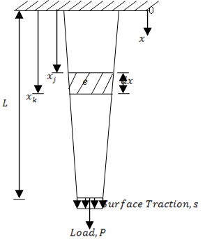
Figure 1. Suspended Column under Applied Load
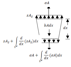
Figure 2. Elemental Portion of the Column
Resolving the forces on elemental volume of the uniaxial stress column in static equilibrium in the x-direction, we have:
|
|
(2) |
Equation (2) reduces to:
|
|
(3) |
Solving equation (3) using the finite element method by adding the weight function [8,9]:
|
|
(4) |
Considering only linear elastic material for which the constitutive. The stress-strain relationship for the uniaxial stress state is given by:
|
σ = E(ε-ε0) + σ0 |
(5) |
Assuming there no pre-stress, σ0, and self strain, ε0 = αTΔT, due to thermal expansion in the material. Therefore, the constitutive relationship is a somewhat more general form of Hooke’s law:
|
σ = Eε, where ε = du/dx |
(6) |
Substituting (6) in (4) and resolving first term of equation through integration by parts:
|
|
(7) |

The vector of nodal unknown for an element is related to local nodal displacements uj and uk at nodes j and k as:
|
|
(8) |
The strain nodal displacement matrix and the global nodal displacements are denoted by B = LN and u =Naε therefore:
|
Ε = Baε |
(9) |
When L = d/dx the shape function is:
|
|
(10) |

From BT = LNT also substituting in equations (8-10), by replacing with elemental volume dV=Adx, and applying the Gauss Divergence Theorem on the third term of equation (7), we have:
|
|
(11) |

Rearranging equation (11) in the form of kεaε=fε, where kε is the element stiffness matrix and fε is the element nodal vector, it result:
|
|
(12) |

Therefore, from equation (12), we may derive followings:
|
|
(13) |
where:
|
|
(14) |

and:
|
|
(15) |
The average strain, average stress and average load for each element of the column can be computed from equations (15).
Results and Discussion
A graphical user interface (GUI), Figure 3, was developed programmatically using the MATLAB M-File editor to solve the finite element model. Also an About-Program Interface was also created as shown in Figure 4. The Program can solve for suspended column (one end fixed and other end free) with up to 1000 nodes on a computer with Dual-Core 2.0GHz processor and 2GB RAM.
The input parameters with the material properties of Steel AISI CI020 (hot-worked) used to test and validate the MATLAB GUI are listed in Table 1.
The column average strain, average stress and average load are equivalent but more accurate to the ones obtained when the whole column is taken as one element (two nodes for one dimensional linear finite element problem). Table 2 shows the result for two nodes and 20 nodes with no surface traction and body force.
The result of the finite element model for uniaxial stress in column, having twenty nodes, was validated with the exact solution given by Stasa [8] for applied load without surface traction and body force. The axial displacement was found to be in agreement with the exact solution as shown in Figure 5.
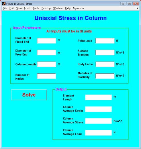
Figure 3. The Graphical User Interface Developed with MATLAB
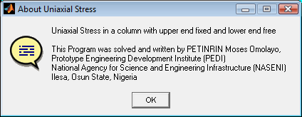
Figure 4. The About-Program Interface
Table 1. The Input Parameter for the MATLAB GUI
|
Parameter |
Value (unit of measurement) |
|
Length of the Column |
0.6 (m) |
|
Length of the Fixed End |
0.1 (m) |
|
Length of the Free End |
0.075 (m) |
|
Applied Point Load |
1500 (N) |
|
Surface Traction |
5000000 (N/m2) |
|
Body Load |
77008.5 (N/m3) |
|
Modulus of Elasticity |
20.7 × 10¹⁰ (N/m2) |
Table 2. Results obtained from Two-Node and Twenty-Node Columns
|
Nodes |
Length |
Average Load |
Average Stress |
Average Strain |
|
2 |
0.6 |
1500 |
249451.0128 |
1.2051∙10-6 |
|
20 |
0.6 |
1500 |
254632.8071 |
1.2301∙10-6 |
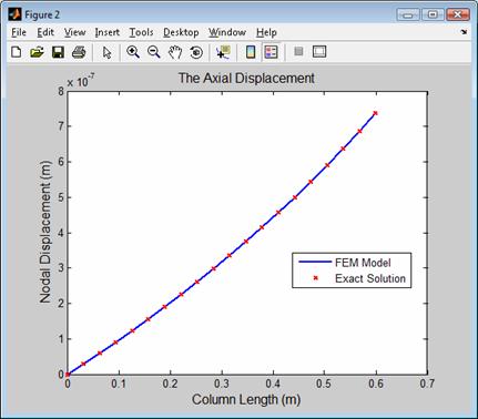
Figure 5. Graph of Nodal Displacement against Column Length
Apart from the results obtained on the GUI, the results of the global stiffness matrix, global nodal force vector, nodal displacements, the element strain, elemental stress and elemental average load on the column are saved in separate text files once the ‘Solve button’ is clicked with left mouse. The results for the stress, strain and applied load distribution are shown in Figure 6, Figure 7 and Figure 8 respectively. It was shown in the three figures that the contribution of the body force, b is insignificant compare to that of the surface traction, s. From Figure 8, the applied load on each elemental portion of the column remains the same because the applied load acting at the nodes within the column cancels each other by that of the adjacent elements or by restrained end will not enter the formulation.
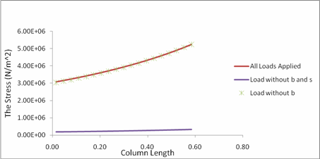
Figure 6. Graph of the elemental Stress Distribution against the Column Length
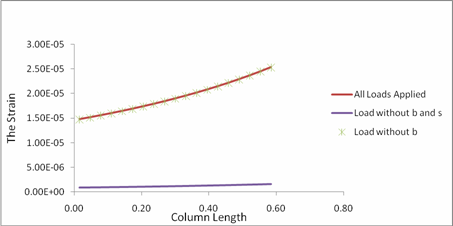
Figure 7. Graph of the elemental Strain Distribution against the Column Length
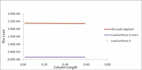
Figure 8. Graph of the Load Distribution against the Column Length
It can also be observed that the body force made a little contribution to the applied load since the diameter at the fixed and is more that that at free end, therefore the weight addition will not be the same.
Conclusions
It has been established from this work that MATLAB is not only a software package for numerical computation but also for application development. The graphical user interface was successfully developed to study the behaviour of suspended column under uniaxial static loading by analysing the governing equation with finite element method (FEM).
The comparison between the exact solution from previous researches and the numerical analysis showed good agreement. The column average strain, average stress and average load are equivalent but more accurate to the ones obtained when the whole column is taken as one element (two nodes for one dimensional linear finite element problem). Stress-strain curves can also be made from the graphical user interface by varying the applied loads for the same material.
References
1. MathWorks, Getting Started with MATLAB, The MathWorks, Inc., Natick, 2007
2. Wikipedia, MATLAB, Wikipedia Foundation Inc; 2010, Retrieved 24th April, 2010 from http://en.wikipedia.org/wiki/MATLAB
3. Buckhale G., Prototype of a computerized system to automatically supply the parameters needed to compute 95% confidence intervals for chemical (and other) measurements (in both biased and unbiased measurement form), AES Bioflux, 2010, 2(2), p. 121-170.
4. MathWorks, MATLAB Creating Graphical User Interfaces, The MathWorks, Inc., Natick, 2007
5. Wikipedia, Stress (Mechanics), Wikipedia Foundation Inc; 2010, Retrieved 28th February, 2010 from http://en.wikipedia.org/wiki/Stress_(mechanics)
6. Case J., Chilver L., Ross C.T.F., Strength of Materials and Structures, 4th edition, Arnold, London, 1999.
7. Nash W.A., Schaum’s Outline Series of Theory and Problems of Strength of Materials, 4th edition, McGraw Hill, New York, 1998.
8. Stasa F.L., Applied Finite Element Analysis, 3rd edition, CBS Publisher, Tokyo, 1985.
9. Zienkiewics O.C., Taylor R.L., The Finite Element Method, 5th edition, vol. 1, Butterworth-Heinemann, Barcelona, 2000.