A New Intelligent Scheme for Simultaneous Cold Junction Compensation and Linearization of Thermocouples
Debangshu DEY and Sugata MUNSHI*
Department of Electrical Engineering, Jadavpur University, Kolkata-700032, India.
E-mail(s): debangshudey80@gmail.com; sugatamunshi@yahoo.com
* Corresponding author: Phone: +913324146949
Abstract
The paper presents a novel neural network based system for processing thermocouple signals, performing the tasks of linearization of the sensor transfer curve and cold junction compensation in the same stride. Keeping an eye on the viability of the complete system as a commercial product, a thermistor has been considered for sensing the reference junction temperature. Cost of the remaining hardware is also minimal. With the use of versatile Differential Evolution (DE) algorithm during the training of a multilayered Artificial Neural Network (ANN) to initialize the weight and biases of the ANN, it has been possible to achieve remarkably low measurement errors, as revealed by the simulation studies.
Keywords
Thermocouple; Cold Junction Compensation; Linearization; Artificial Neural Network.
Introduction
Accurate measurement of temperature is one of the most common and vital requirements in industrial instrumentation. It is also one of the most difficult objectives to achieve. Unless proper temperature measuring techniques are employed, serious inaccuracies of reading can occur, or may result in useless data. For this purpose, several instruments have been devised to measure temperature correctly and the well-known of them is the mercury thermometer. Current interest ranges from cryogenics (a few Kelvin) to plasma (10,000 K upwards). However, most applications are in the range of room temperature to 2000 K [1]. The thermocouple is by far the most widely used temperature sensor for industrial instrumentation. Its favourable characteristics include good inherent accuracy, suitability over a broad temperature range, relatively fast thermal response, ruggedness, high reliability, low cost (except for the noble metal thermocouples), and great versatility of application in the sense that the thermocouple group of sensors can be optimized for a variety of environmental conditions. The main limitation is accuracy; as system errors of less than 1°C may be difficult to achieve [1-5]. In most cases, sensor outputs are nonlinearly related to the physical variables they sense, and thermocouples are no exception. They also generate voltage signals that are nonlinearly related to temperature being measured. For solving this problem the sensor output requires correction. Another important issue in the processing of thermoelectric signals is the cold junction compensation (CJC), which calls for maintaining the reference junction temperature at 0ºC or simulating a similar condition by electronic or other methods [3-5,11]. While many of the generalized hardware and software based linearization techniques can also be used for thermocouples, some have been specifically applied for this class of sensors [7-9]. In those works, the reference junction has been assumed to be held at a constant temperature of 0ºC. Several development works on cold junction compensation have also been reported [5, 10, 11]. Commercially available hardware modules, e.g. SCM7B47 from DATAFORTH, which perform both cold junction compensation and linearization for different types of thermocouples, are also available. Obviously for such systems, with a change in the type of thermocouple used, the module also has to be replaced.
In this work, an artificial neural network (ANN) was proposed as a tool to linearize the characteristics of different thermocouples.
Material and Method
The ANN is fitted to the calibrating data with a desired final error. In this work we have used evolutionary algorithm based Differential Evolution (DE) algorithm for ANN training. Thus the weights and biases of the network are initialized with DE and thereafter this initialized network is again retrained with the help of Levenberg-Marquadt algorithm. Provision for cold junction compensation (CJC) is also integrated with the ANN linearizer and uses the data related to the reference junction temperature from a circuit employing a thermistor with negative temperature coefficient (NTC). It is worth mentioning that linearization of thermocouple characteristics by using ANN is nothing new, but the novelty of the present work lies in the fact that it presents an ANN based technique that serves the dual purpose of linearization and cold junction compensation.
The proposed scheme has been tested by MATLAB based simulation using the manufacturer’s data for J and K type thermocouples having decent linearity and also for G type thermocouple whose characteristic is the most nonlinear and non-monotonic as well.
An Overview of Linearization and Cold Junction Compensation Techniques
Linearization of sensor characteristic plays a vital role in electronic instrumentation because all sensors have outputs nonlinearly related to the physical variables they sense. If the sensor output is nonlinear, it will produce a whole assortment of problems [5, 6, 10]. A variety of analog circuits are used for sensor linearization [13], which implies additional analog hardware and the typical problems associated with analog circuits (e.g. error due to temperature drift). If the system includes a microprocessor or a computer, we can cope with the sensor non-linearity by means of arithmetic operations, if a reasonably accurate sensor model is available. Another possibility is the use of a look-up table, which may require a considerable amount of memory for enhanced accuracy, resulting in a problem in small microprocessor systems or microcontrollers.
The conceptually simplest way of cold junction compensation is to keep the reference junction of the thermocouple immersed in a carefully constructed ice bath (i.e. at 0ºC) and the voltage measuring device can be comfortably calibrated in terms of the sensing junction temperature. However maintenance of the ice bath in industrial environment being a problem, people look for alternatives. One approach is to use two temperature controlled ovens maintained at two different temperatures to simulate the effect of a 0ºC reference junction temperature. Principle of the electronic methods in current use is to employ an auxiliary sensor for sensing the reference junction temperature, and the sensor output is electronically processed to generate an appropriate voltage which is combined with the thermocouple output to yield a cold junction compensated output. In more sophisticated systems, a voltage related with the reference junction temperature is developed by a sensor as stated above and this voltage and the thermocouple output are processed by software with an appropriate numerical algorithm to yield the temperature being measured. Thus, the software performs the task of linearization and cold junction compensation in the same stride. The scheme presented in this paper is a variant of this approach. The procedure utilizes a simple multi-layered ANN as in [8, 12].
An Improved Scheme for Simultaneous Linearization and Cold Junction Compensation
The proposed measurement scheme is shown in figure 1. As evident from the figure, in this proposed scheme the reference junction of the thermocouple is at the ambient temperature Ta. This ambient temperature may vary and usually not at 0°C. So the NTC thermistor arrangement will serve the purpose of an extra sensor to sense the ambient temperature.
The thermistor is placed in series with a known constant resistance. The series circuit is fed from a constant voltage source (Vi). The voltage drop across the constant resistance (r) is measured. As temperature increases, the resistance of the thermistor (RT) decreases. So the circuit current and the voltage drop across the resistance r will increase.
It is easily understood that this voltage is a function of ambient temperature. Therefore this voltage Eo(Ta) can be utilized for cold junction compensation. The thermocouple output voltage is V0 (Td), where Td = TS – Ta, TS being the temperature under measurement.
The voltage V0(Td) and E0(Ta) are captured by a computer based data acquisition system, where they are digitized and then processed by a neural algorithm. It is intended that the neural network will predict the temperature TS under measurement from the values of V0 and E0 (which depends on the cold junction temperature) as inputs and T0 as the target. On completion of the training, the ANN linearizer is ready to calculate TS from the measured values of V0 and E0.
The expression for the thermistor circuit voltage, as evident from figure 1, is given by:
|
|
(1) |

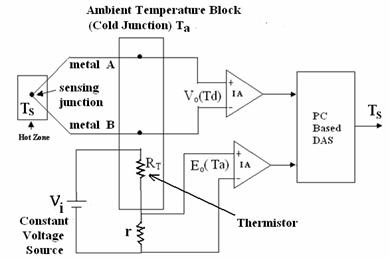
Figure 1. Proposed Measurement Scheme
This arrangement has an added advantage that it provides a series linearizing scheme for the thermistor. To utilize the linearizing action of the series resistance the value of r is judiciously chosen. This reduces the task of the ANN linearizer to a certain extent. The well-known expression for the value of linearizing series resistance is [13]:
|
|
(2) |

Here, we have considered the approximate characteristic equation of the thermistor given by:
|
|
(3) |
where: RT = resistance of thermistor at temperature T in Kelvin; RT0 = Resistance of thermistor at temperature T0 in Kelvin; β = a constant between 1500K to 7000K depending upon the type of thermistor; TM = midpoint of the temperature range over which the thermistor is to be used; RTM = resistance of thermistor at temperature TM in Kelvin.
The value of β is obtained from the equation given below by the method of least squares as:
|
|
(4) |

where: RTi = thermistor resistance at Ti Kelvin and n = number of data points considered.
|
|
(5) |
The constant input voltage (Vi) is determined considering the heat dissipation capability of the thermistor package. As the transfer characteristics of the thermocouples and the resistance-temperature characteristic of a NTC thermistor are both nonlinear, the importance of a linearizing scheme for this proposed arrangement is immense.
The ANN Signal Processor
Artificial neural networks (ANN) are processing elements based on the principle of work of human brain [14, 15]. An ANN consists of a set of artificial neurons (processing units), and their connections (which are so called weights and biases). ANN learns, i.e adjusts its weights and biases, from input-output data called examples. As ANNs are model-free estimators, it is not necessary to presume a model function that relates the input-output data pairs. Artificial neural networks are extensively useful in a wide spectrum of applications such as signal and image processing, pattern recognition [16], control systems [17] and instrumentation also [18]. As ANNs possess nonlinear characteristics, they are very useful in solving complex and nonlinear problems. They provide better and more accurate results as compared to linear techniques. Among the various applications of ANNs, Hofer et al [19] have envisaged a neural network that can successfully control the strip thickness of a steel rolling mill. In power systems also [17] an adaptive variable structure voltage regulator is implemented using an artificial neural network.
In the present case, a multi-layered (2-15-1) feed forward neural network has been considered (as shown in figure 2). It has input layer with two input node, a hidden layer ANN with twenty nodes and output layer with two nodes. Each hidden node multiplies every input by its weight and sums the product and then passes the sum through the sigmoid function. The outputs from the output layer of the neural network are compared to the target value of the training data function to calculate the error. Differential Evolution (DE) algorithm has been used for initializing the weights and biases of the ANN [20-22], and thereafter this initialized network is again trained with the help of Levenberg-Marquadt algorithm [23-25].
Figure 2. Structure of Artificial Neural Network
Results and Discussion
The simulation and testing of the scheme has been carried out using SIMULINK and Neural Network Toolbox of MATLAB 6.5 in a Pentium 4 processor based PC. UUA 33J4 thermistor of Omega Engineering has been considered as cold junction temperature sensor and its resistance-temperature data obtained from the manufacturer [26] have been utilized for simulation.
During training of the ANN, 100 epochs (iterations) have been used for initialization of the weights and biases of the network by DE algorithm and the initialized network is then trained using 350 epochs (iterations) with Levenberg-Marquadt algorithm. A new program TRAINDE.m has been used to implement the DE algorithm for training the ANN, and conventional MATLAB function trainlm is used for training the ANN using Levenberg-Marquadt algorithm.
The ambient temperature has been considered to vary from 0ºC to 50ºC. Hence TM=25ºC. For the thermistor under consideration, RTo=3000Ω at reference temperature T0=298K. The value of β has been obtained from equation (4) as 3961.8K, by considering 51 data points (i.e. n=51), 1°C apart, over the temperature range of interest. Since the heat dissipation capability of the thermistor package is 0.1 mWatt, a safe value of the supply voltage Vi is taken as 1 volt. To utilize the linearizing action of the series resistance, the value of r is chosen as 2516.92Ω, as obtained from equation (2).
The percentage full scale (FS) error for each type of the thermocouple has been calculated. These results are shown in tables 1-4, as well as in figure 3-10). As G thermocouple has a unique non monotonic characteristic, performance of the scheme has been evaluated for two different ranges of operations (0–2300ºC and 250–2300ºC) for this thermocouple. The extremely low value of errors proves the effectiveness of the scheme.
Table 1. Percentage Full-scale Error for K Thermocouple for Different Ambient Temperature
|
Thermocouple Type |
Measured Temperature Range (oC) |
Ambient Temp. (oC) |
Max. Error (+ve) (% FS) |
Max. Error (-ve) (%FS) |
RMS Error (%FS) |
|
K |
0 - 400 |
0 |
0.00042 |
0.00036 |
0.000009 |
|
10 |
0.00057 |
0.00064 |
0.000065 |
||
|
20 |
0.00046 |
0.00056 |
0.000087 |
||
|
30 |
0.00033 |
0.00028 |
0.000029 |
||
|
40 |
0.00025 |
0.00049 |
0.000057 |
||
|
50 |
0.00034 |
0.00046 |
0.000066 |
Since type K thermocouple has a transfer curve with quite good linearity, its entire application range has not been considered. As expected, the proposed scheme has been found to work brilliantly for this thermocouple.
Table 2. Percentage Full-scale Error for J Thermocouple for Different Ambient Temperature
|
Thermocouple Type |
Measured Temperature Range (oC) |
Ambient Temp. (oC) |
Max. Error (+ve) (% FS) |
Max. Error (-ve) (%FS) |
RMS Error (%FS) |
|
J |
0 - 750 |
0 |
0.000035 |
0.000021 |
0.0000037 |
|
10 |
0.000041 |
0.000050 |
0.0000043 |
||
|
20 |
0.000033 |
0.000038 |
0.0000013 |
||
|
30 |
0.000039 |
0.000022 |
0.0000011 |
||
|
40 |
0.000027 |
0.000024 |
0.0000082 |
||
|
50 |
0.000011 |
0.000045 |
0.0000041 |
For J type thermocouple, whose transfer curve is less linear, the error reported in literature is ± 0.29% over OºC to 300ºC. The prediction error obtained with the present scheme is within ± 0.45 × 10⁻⁴ % over 0ºC to 750ºC which is indeed a remarkable feat to achieve.
For the G type thermocouple, it has been reported by various researchers that over 250ºC to 2150ºC, the RMS errors are obtained as 2.11ºC, 1.27ºC, 1.06ºC with linear interpolation, quadratic interpolation and an ANN method respectively. In the present work, over a similar range of temperature, the maximum RMS error is obtained as 0.000046% of full scale, which corresponds to 0.0011°C. Even for wider range (i.e. 0°C to 2300°C) the maximum RMS error is 0.00087% of full scale, i.e. 0.002°C. This achievement of the proposed scheme can be considered to be really exceptional, considering the non-monotonic transfer curve of the thermocouple which makes the transducer less amenable to linearization.
Table 3. Percentage Full-scale Error for G Thermocouple (in the range 0-2300oC) for Different Ambient Temperature
|
Thermocouple Type |
Measured Temperature Range (oC) |
Ambient Temp. (oC) |
Max. Error (+ve) (% FS) |
Max. Error (-ve) (%FS) |
RMS Error (%FS) |
|
G |
0 - 2300 |
0 |
0.00125 |
0.00030 |
0.000067 |
|
10 |
0.00087 |
0.00054 |
0.000063 |
||
|
20 |
0.00037 |
0.00037 |
0.000087 |
||
|
30 |
0.00041 |
0.00026 |
0.000022 |
||
|
40 |
0.00045 |
0.00039 |
0.000060 |
||
|
50 |
0.00022 |
0.00055 |
0.000047 |
Table 4. Percentage Full-scale Error for G Thermocouple (in the range 250oC - 2300oC) for Different Ambient Temperature
|
Thermocouple Type |
Measured Temperature Range (oC) |
Ambient Temp. (oC) |
Max. Error (+ve) (% FS) |
Max. Error (-ve) (%FS) |
RMS Error (%FS) |
|
G |
250 - 2300 |
0 |
0.00031 |
0.00049 |
0.0000270 |
|
10 |
0.00028 |
0.00044 |
0.0000220 |
||
|
20 |
0.00033 |
0.00054 |
0.0000460 |
||
|
30 |
0.00042 |
0.00046 |
0.0000433 |
||
|
40 |
0.00024 |
0.00036 |
0.0000410 |
||
|
50 |
0.00024 |
0.00048 |
0.0000213 |
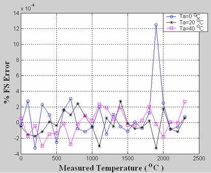
Figure 3. %FS Error variation for G thermocouple with change in Measured Temperature (Ts) for different Ambient Temperature (Ta) [for the range 0°C–2300°C for Ts]
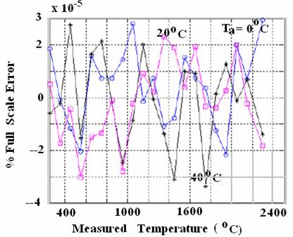
Figure 4. %FS Error variation for G thermocouple with change in Measured Temperature (Ts) for different Ambient Temperature (Ta) [for the range 250°C–2300°C for Ts]
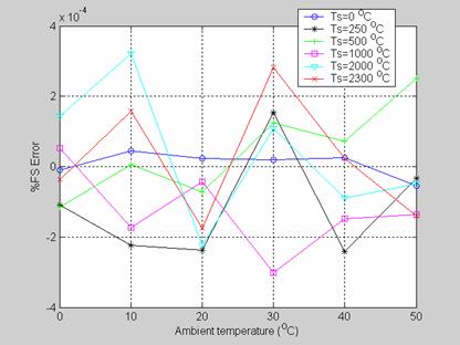
Figure 5. %FS Error variation for G thermocouple with varying Ambient Temperature (Ta) for different values of Measured Temperature (Ts) [in the range of 0°C– 2300°C]
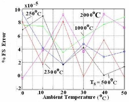
Figure 6. %FS Error variation for G thermocouple with varying Ambient Temperature (Ta) for different values of Measured Temperature (Ts) [in the range of 250°C– 2300°C]
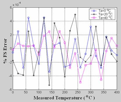
Figure 7. %FS Error variation for K thermocouple with change in Measured Temperature
(Ts) for different Ambient Temperatures (Ta)
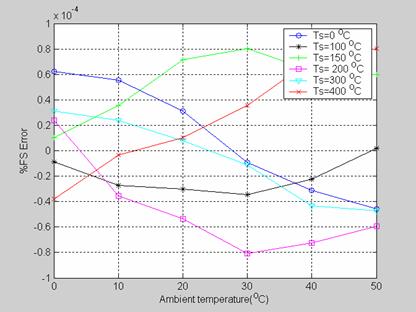
Figure 8. %FS Error variation for K thermocouple with varying Ambient Temperature (Ta) for different values of Measured Temperature (Ts)
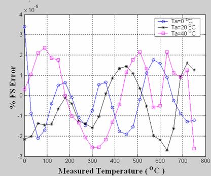
Figure 9. %FS Error variation for J thermocouple with change in Measured Temperature (Ts) for different Ambient Temperature (Ta)
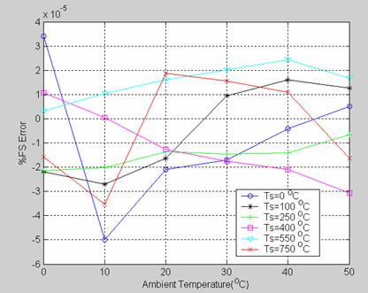
Figure 10. %FS Error variation for J thermocouple with varying Ambient Temperature (Ta) for different values of Measured Temperature (Ts)
Conclusions
An ANN based signal conditioning arrangement has been devised for thermocouples, which performs the dual task of compensating the transfer-curve nonlinearity as well as the error due to drift in the temperature of the reference junction. The weights and biases of the neural network have been optimized by a versatile evolutionary algorithm. The performance of the system as assessed by simulation is superb. It is by far superior to those schemes developed earlier. It is worth mentioning that these earlier thermocouple signal processing arrangements were meant to serve as linearizers only and conventional hardware methods were considered for CJC.
An attractive feature of the present scheme is the use of a very low-cost sensor (thermistor) for sensing the reference junction temperature. It is also to be noted that if the thermocouple type is changed due to any reason, the system can be adapted for the changed situation, simply by retraining the neural network, or at most a change in the structure of the network has to be introduced.
When visualized as a compact commercial product, the system will consist of the thermistor, the associated electronic circuitry and a microcontroller based system programmed with the ANN software. With the rapid development of ANN chips, such ICs can also be utilized.
References
1. Considine D.M., Process Instruments and Controls Handbook, McGraw-Hill, New York, 1985.
2. Dahl A.I., Temperature, Its Measurement and Control in Science and Industry, Reinhold Publishing Corporation, Chapman & Hall Ltd. London, 1962.
3. Doebelin E.O., Measurement System Application and Design, McGraw-Hill Publishing Co,New York, 1990.
4. Dalley J.W., Riley W.F., McConnell K.G., Instrumentation for Engineering Measurements, John Wiley & Sons, 1993.
5. Preobrazhensky V.P., Measurement and Instrumentation in Heat Engineering, MIR Publishers, Moscow, 1980.
6. Wang X., Wei G., Sun J., Free knot recursive B-spline for compensation of nonlinear smart sensors, Measurement-Elsevier, 2011, 44 (5), p. 888-894.
7. Ximin L., A Linear Thermocouple Temperature Meter Based on Inverse Reference Function, International Conference onIntelligent Computation Technology and Automation (ICICTA 2010), 2010, 1, p. 138 - 143.
8. Sarma U., Boruah P.K., Design and development of a high precision thermocouple based smart industrial thermometer with on line linearisation and data logging feature, Measurement-Elsevier, 2010, 43 (10), p. 1589-1594.
9. Wang D., Song L., Zhang Z., Contact temperature measurement system based on tungsten-rhenium thermocouple, International Conference on Computer Application and System Modeling (ICCASM 2010), 2010, 12, p. 660 - 663.
10. Danisman K., Dalkiran I., Celeb F.V., Design of a high precision temperature measurement system based on artificial neural network for different thermocouple, Measurement-Elsevier, 2006, 39 (8), p. 695-700.
11. Han B.; Liu L., He C., Du L., Application of ANN on the Intelligent Temperature Sensor, The Sixth World Congress on Intelligent Control and Automation ( WCICA 2006), 2006, 1, p.4956 - 4959.
12. Dalkiran I., Danisman K, Linearizing E-Type Thermocouple Output Using Artificial Neural Network and Adaptive Neuro-Fuzzy Inference Systems, IEEE 14th Signal Processing and Communications Applications, 2006, p.1 - 4.
13. Tietze U., Schenk Ch., Electronic Circuit Design and Applications, Narosa Publishing House, New Delhi,1992.
14. Haykin S., Neural Networks, A Comprehensive Foundation, Macmillan, 1994.
15. Martin del Brio B., Sanz Molina A., Neural Networks and Fuzzy Systems, RAMA, Madrid, 1997.
16. Freeman J.A., Neural Networks: Algorithms, Applications, and Programming Techniques, Addison-Wesley, Massachusetts, 1992.
17. Aggoune M.E., Boudjema F., Bensenouci A., Hellal A., Vadari S.V., El Mesai M.R., Design of an Adaptive-Structure Voltage Regulator Using Artificial Neural Networks, Proc. of the 2nd IEEE Conference on Control Applications, Vancouver, Canada, September 1993, p. 337-343.
18. Chudzik S., The idea of using artificial neural network in measurement system with hot probe for testing parameters of heat-insulating, Measurement-Elsevier, 2009, 42(5), p. 764-770.
19. Hofer D.S., Neumerkel D., Hunt. K., Neural Control of a Steel Rolling Mill, IEEE Transactions on Control Systems, June 1993, p. 69-75.
20. Ilonen J., Kamarainen J.K., Lampinen J., Differential Evolution Training Algorithm for Feed-Forward Neural Networks, Neural Processing Letters, Kluwer Academic Publishers, 2003, p. 93-105.
21. Storn R., Price K., Differential Evolution - A Simple And Efficient Heuristic for Global Optimization Over Continuous Spaces, Journal of Global Optimization,1997, 11(4) , p. 341-359.
22. Zelinka I., Lampinen J., An Evolutionary Learning Algorithm for Neural Networks, 5th International Conference on Soft Computing, MENDEL'99, 1999, p. 410-414.
23. Magoulas G.D., Plagianakos V.P., Vrahatis M.N., Hybrid Methods Using Evolutionary Algorithms for On-Line Training, Proc. of the IEEE International Joint Conference on Neural Networks, IJCNN 2001, Washington DC, USA, 2001, 3, p. 2218-2223.
24. Charalambous C., Conjugate Gradient Algorithm for Efficient Training of Artificial Neural Networks, Proc. IEE (Circuits, Devices and Systems), 1992, p. 301-310.
25. Masters T., Land W., A New Training Algorithm for the General Regression Neural Network, IEEE International Conference on Systems, Man, and Cybernetics, Computational Cybernetics and Simulation ,1997, 3, p. 1990-1994.
26. Temperature Measurement Handbook, Omega Engineering Inc., Stanford, Connecticut, 1979.