Dynamic Thermal Rating for Overhead Lines:
Self-adaptive Protection Device
Fabio MASSARO1*, Rosario MICELI1, and Renato RIZZO2
1 DEIM - Università di Palermo, Viale delle Scienze, 90128 Palermo, Italy
2 DIETI - University of Naples Federico II, Via Claudio 21, 80125 Naples, Italy
E-mails: fabio.massaro@unipa.it*; rosario.miceli@unipa.it; renato.rizzo@unina.it
* Corresponding author: Phone: +39 9123860295; Fax: +39 916197439
Abstract
The increase in the consumption of electricity, the stringent environmental restrictions and the need to keep costs, make ever more meaningful the need for a flexible operation of existing overhead lines. This paper studies the possibility to use a dynamic thermal rating for overhead line starting from the analysis of the mathematical model and the ability of the latter to reflect the temperature of an overhead conductor in different ambient condition; then it simulates the thermal behaviour of a conductor both in steady state and dynamic one. Finally the paper shows a method for a self-adaptive thermal protection system.
Keywords
Dynamic thermal rating; Thermal behaviour of overhead line; Self-adaptive protection device; Overhead conductor; Ampacity.
Introduction
Among many factors that limit the power transmitted in an overhead line, the maximum allowable temperature for the conductors can sometimes become one of the more restrictive conditions, especially for short lines.
The temperature rise of the conductors determines:
¸ the relaxation of the conductors with the consequent increase of the sag in each span (risk of discharge);
¸ a reduction of mechanical and electrical properties of the conductors.
The transmission system has the task of ensuring the dispatch of energy from generators to consumption ensuring adequate levels of safety and economy, while maintaining high standards of service quality also considering the diffusion of distributed generation systems with renewable sources [1-4].
Considering the recent deregulation of energy markets, today assumes great importance the ability to ensure the transfer of energy freely contracted between a set of producers (domestic and foreign) and a set of clients variously located in the system. The exceeding of the limits of capability of one or more lines can make incompatible the power flows, consequently causing the inhibition of some exchanges, even if, already bilaterally agreed by contract. To up rate a line is possible:
¸ to make a re-conductoring (conductor replacement) of the line with low-sag-high-temperature components [5];
¸ to exploit favourable ambient conditions [6].
The operation of the system can be affected by [7-11]:
¸ the unavailability of a line, which requires a redistribution of power flows on the other conductors in the system;
¸ the sudden outage of a substantial part of the generation which undertakes to transfer power from the surrounding areas.
The approach, up to now followed, is static; it assess the carrying capacity of an overhead power line based on environmental conditions "reasonably the worst", and defines the maximum power transmitted from a power line. It is clear that this type of approach, considering the above considerations, it is inadequate to the new requirements of flexibility that the transmission network has to ensure.
The limits of such approach regard, above all, the inability to follow the changes in weather conditions and to provide the margin of overload in emergency conditions to ensure wider safety margins; these limits, in particular ambient conditions, do not exclude the risk of thermal overload.
A dynamic control system of the conductor temperature makes possible to solve the above problems and provides the following advantages:
¸ increasing the average power transmitted;
¸ report overload conditions;
¸ flexible operation of the transmission network that allows to postpone the construction of new lines or upgrading of existing ones;
¸ lower thermal stress for the conductors;
The implementation of a real-time control system of the temperature is based on a mathematical model which takes into account all important parameters that determine changes in temperature of the conductor such as: temperature, wind speed and direction, etc.
The real time control needs a prediction of the environmental conditions in the short period; the development of mathematical models of the atmosphere and the use of adaptive filters (based on mathematical models of the type balanced input-state-output state feedback as the Kalman filter) which, by rearranging the observed data and their series, provides forecasts up to 24 hours, combined with stochastic models for the prediction of thermal boundary flow of overhead power lines, allow the programming of network structures and plans daily production [12-14].
The aim of this research was modelling a dynamic system for the up rating of overhead lines according to favourable ambient conditions to maximize the ampacity of conductors.
The Mathematical Model
The heat balance equation of a conductor consists of more terms, which contribute, in a different way, to the variation of its temperature. The model presented here refers to a span (ideal) for which, all along, both the environmental conditions and the physical characteristics, shall be considered as constants; the conductor is considered:
¸ homogeneous and isotropic, of cylindrical shape and horizontal axis;
¸ having a diameter equal to the cross section of the real conductor;
¸ having an infinite thermal conductivity;
¸ crossed by alternating current at 50 Hz uniformly distributed over the section;
¸ free from singularities such as joints and elements of the terminal box and free from influences end, other conductors or surrounding objects.
It’s important to take into account the radial temperature distribution within a conductor; a complex method to calculate the radial temperature distribution in stranded conductors is given in [15]. Due to the fact that the difference between the core and the surface temperature is quite small, it’s generally sufficient to assume that the temperature of the surface is about the average temperature of the conductor [16].
The equation that governs this phenomenon is the following [17]:
|
|
(1) |
Where: m – specific mass of the conductor, cp – the specific heat of the conductor, Qgen - the heat generated by Joule effect, Qsun - the heat absorbed by solar radiation, Qrad - the heat lost by radiation, Qconv - the heat lost by convection.
Formula (1) shows how the accumulated heat in the conductor, which is the first member, is equal to the difference between absorbed and lost heat. These terms will be individually examined to highlight their dependence on environmental conditions.
a) Qgen depends on the characteristics of the electrical conductor and in particular by its AC electrical resistance. Its expression is:
|
|
(2) |
where: R20°C - AC resistance of the conductor at a temperature of 20 °C; α - the temperature coefficient of resistance; T(t) - the temperature of the conductor; I(t) - the current flowing in the conductor.
b) Qsun is the heat gained by solar radiation; it depends on both the direct radiation of the sun and the diffuse one from the environment. Its expression is:
|
|
(3) |
where: D - diameter of the conductor; αs, α1 - solar absorptivity, direct and reflected; Qdir, Qdiff - the amount of heat absorbed for direct and diffuse radiation.
Considering that experimental measurements have shown that the amount of heat gained by solar radiation influences for a few Celsius degrees, compared to the heat produced by the Joule effect, it is preferred to estimate Q*sun = Qdir equal to 1000 W/m2 (neglecting the term Qdiff almost irrelevant for the purposes of the study). This value, referring to a summer's day and not taking into account the screening of the clouds, it can be considered conservative; the expression of Qsun becomes:
|
|
(4) |
where the solar absorptivity can be obtained from infrared emission coefficient ε by the following equation:
|
|
(5) |
with the restriction that αs <1.
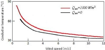
The figure 1, from [18], shows the trend of the temperature of the conductor varying the speed of the wind, with and without solar radiation; the temperature increase due to is modest, for high values of the wind speed.
|
|
|
Figure 1. Conductor temperature varying the wind speed, with and without solar radiation |
c) Qrad is the amount of heat lost by radiation from the surface of the conductor. Its expression is:
|
|
(6) |
where: ε - is the emissivity of the conductor that can be put in relation with the age y, in years, of it by the following experimental expression, valid for ACSR conductors:
|
|
(7) |
σ – is the Stefan-Boltzmann constant, σ =5.6697·10-8; Ta(t) - the ambient temperature.
Qrad, as Qsun, is of limited importance in the determination of the thermal equilibrium of a conductor, in fact, its percentage contribution decreases with increasing wind speed.
d) Qconv is the amount of heat lost by convection, its expression is:
|
|
(8) |
where: h(t) - the heat transfer coefficient that depends on the intensity and direction of the wind, the air and conductor temperature. The expression of h(t) is:
|
|
(9) |
where: K - is the radial thermal conductivity assumed, K=0.026; Nu - the Nusselt number.
The analytical expression of the Nusselt number depends on the intensity of the wind. In conditions of zero wind speed (<0.2 m/s) is:
|
|
(10) |
where: Pr - the Prandtl number, which can be considered constant and equal to 0.71 and the Gr is the Grashof number equal to:
|
|
(11) |
where: β - the coefficient of cubical expansion of the air, β = (273.15)-1; ρ - the air density, ρ = 1.29 [kg/m3]; µ - the viscosity of the air immediately surrounding the conductor that depends on the current: μ = 1.8 10-5 (for I > 700 A); μ = 2.2 10-5 (for 400 <I < 700 A); μ = 2.39 10-5 (for I < 400 A); and g - the acceleration of gravity, g = 9.81 [m/s2].
In windy conditions (> 0.2 m/s) the expression of Nu is independent from temperature and, assuming that the wind is orthogonally to the axis of the conductor, takes the following form:
|
|
(12) |
where: Re - the Reynolds number, n - a coefficient depending on the shape of the conductor and it is assumed to be 0.35; c and m are two coefficients that depend on the shape of the conductor and the Reynolds number, for a cylindrical conductor, is: for Re <1000, c = 0.59, m = 0.47, for Re > 1000, c = 0.665, m = 0.47.
Reynolds number is equal to:
|
|
(13) |
where: ν [m/s] is the wind speed.
If the wind direction is different from that perpendicular to the axis of the conductor, the Nusselt number is multiplied by a term dependent on the angle of incidence of the wind:
|
|
(14) |
where: ω - the angle of incidence of the wind, i.e. the angle between the wind direction and the normal to the conductor. The equation (1), non-linear, cannot be solved in closed form. The resolution was carried out with the method of the fourth order Runge-Kutta, implemented in MATLAB, assuming as initial condition the temperature of the conductor at time t=0. If set to zero the first member of the equation (1); it becomes an algebraic equation that allows to know the steady-state temperature of a conductor for a given current I [18-19].
Matlab Implementation of The Model
To implement the thermal model of a conductor on the simulation software is necessary to rewrite the equation (1) in the following form:
|
|
(15) |
where: C1, C2, C3 are constants and have the following expressions:
|
|
(16) |

The model presented here refers to the condition ν> 0.2 m/s, for which h does not depend on the temperature. The model considers, therefore, a step change of the input variables that determines an approximation of the simulation results, which need to be taken into account in the evaluation of the latter. Tests carried out by CESI on the 380 kV Bovisio-Soazza line, through a system of data acquisition and processing, have shown that the gap between real and calculated temperature is maintained in the range of 5 °C with updates every 5 minutes of the measures. This model can be used to determine the rating of the line under study.
Steady-State Analysis
The thermal rating of a power line refers to the conditions of thermal steady-state; then the analysis will be based on the study of the model at steady-state (i.e. for dT/dt = 0), figure 2. As example it will be considered a 220 kV line equipped with conductors of diameter and section respectively D=22.8 mm and S = 307 mm2, whose characteristics are the following: R20°C = 0.00011 [Ω/m], α = 0.004 [K-1]; Κ = 0.026 [W/mK], ε = 0.854 (y = 10 years); Qsun = 22.8 [W/m]; mcp = 0.229628 [Wh/mK].
|
|
|
Figure 2. Thermal balance in a conductor |
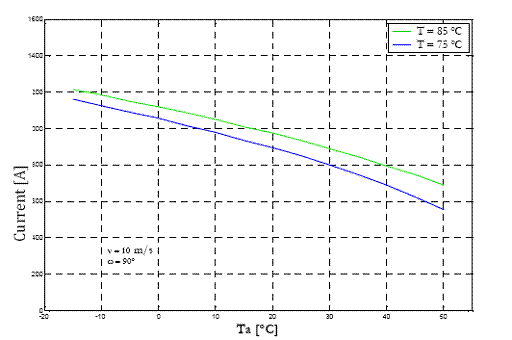
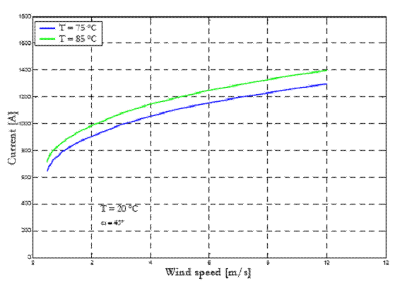
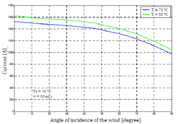
Using the mathematical model, it is shown how the environmental conditions influence, significantly, the thermal rating of the line; figures 3-5 in particular drawn the sensitivity to ambient temperature Ta, wind speed ν, wind direction respect to the normal of the conductor ω.
|
|
|
Figure 3. Ambient temperature influence on the rating of a line |
|
|
|
Figure 4. Wind speed influence on the rating of a line |
|
|
|
Figure 5. Wind direction influence on the rating of a line |
Non-Steady-State Analysis
The study of the transient behaviour of an overhead line is of particular importance since, from the analysis of the results provided by the simulation program; it is possible to determine the limits of uploading of the line in emergency conditions, and the calibration of the protection device.
The following figures (figure 6-9) show a few examples of thermal transients (with initial temperature of 333K approximately 60°C) in different load and environmental conditions; in each example it has been analysed the variation of only one parameter and its influence on the fundamental characteristics of the transient.
In Figure 6 the variable parameter is the ambient temperature; it is clear that this parameter influences the steady-state temperature almost equal to the variation of the parameter itself (i.e.: if the ambient temperature changes by 10 K, the conductor temperature also varies by about 10 K).
|
|
|
Figure 6. Thermal transient of a conductor varying ambient temperature |
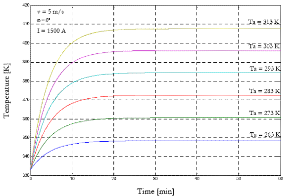
It may also be noted that the thermal time-constant practically does not vary even for large variations of ambient temperature. Figures 7 and 8 are examples related to the change of the speed and wind direction; as already seen for the steady-state analysis, great variations are due to these two parameters also for the transient. In addition, the thermal time-constant increases with decreasing speed, and for angles of incidence close to 90°.
|
|
|
Figure 7. Thermal transient of a conductor varying wind speed |
|
|
|
Figure 8. Thermal transient of a conductor varying wind direction |
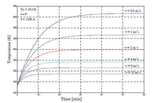
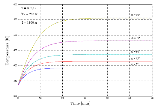
Figure 9, finally, relates to the change of the load current, which significantly influences the steady-state temperature with small variations of the thermal time-constant.
|
|
|
Figure 9. Thermal transient of a conductor varying load current |
Self-Adaptive Protection Device
In this paragraph is shown a strategy for dynamic thermal rating of a line monitoring the thermal overload and setting adequate protection. First it will be illustrated how to obtain time-current curves using the mathematical model and then how to set the calibration of over current protection.
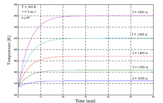
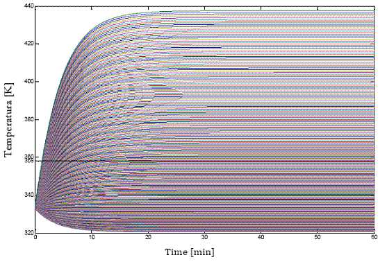
The mathematical model allows to know the thermal transient of a conductor, and so to find the corresponding time-current curve; i.e. how many seconds an overhead conductor takes to reach a temperature Tf (final temperature) for a given current I starting from a temperature Ti (initial temperature), considering constant ambient conditions. Considering a vector of currents, the thermal model derives the time-current curve drawing more thermal transients. The result of the simulation is a family of curves representing different thermal transients; it was considered a wide range of current from 600 A up to1800 A with a step of 5 A; this choice allows to analyse all transient of interest. The next step is to choose what temperature should reach the conductor; in the example of figure 10, it has been chosen Tf = 358 K (85°C).
|
|
|
Figure 10. Thermal transient curves of the vector of currents |
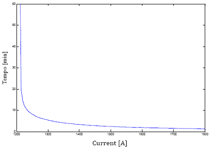
The straight line 358 K intersects the curves, relating to the different currents, at different times; these couples of data (current-time) give the time-current curve. To find the couples of values current-time provided by the curves of figure 10 it is used a simple algorithm implemented in MATLAB. The curve thus obtained is shown in figure 11.
|
|
|
Figure 11. Time-depending curve rating for a conductor |
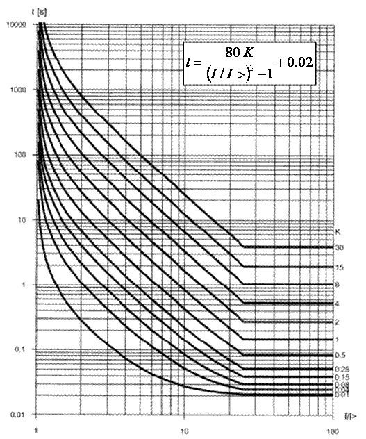
To avoid that a conductor can reach dangerous overheating, it’s possible to set an over current protection where it is possible to implement the time-current curve obtained from the thermal model. The ideal situation would be to transfer to the protection device the time-current curve (i.e. the vector of couples time-current data); as an example of application it has been considered a protection device of digital type that allows to be calibrated from outside via an optical fibre. This type of device has the ability to adjust the first tripping threshold by a family of curves (time-inverse) figure 12, each of which is settable by means of two parameters: I> (threshold current) and K.
|
|
|
Figure 12. Family of curves of the protection device |
To show an example as protection suits the purpose, it tries to fit minimizing the area between the two curves with the restriction that the protection curve always acts before the time-current curve. The result of the simulation is shown in figure 13.
|
|
|
Figure 13. Self-adaptive curve of the protection device to the ambient condition |
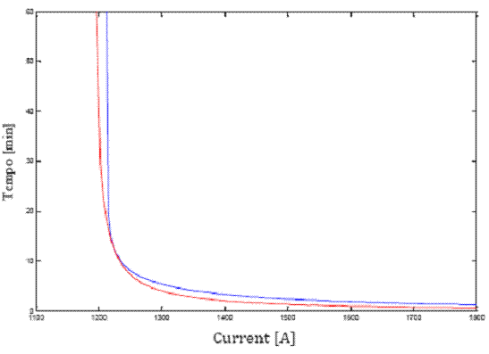
It is evident from the figure that the adaptation is not perfect but the errors are content with variations of 2°C for current close to the capability of the line, and 5-10°C for the highest values of the current (it is clear that the errors are all negative being the protection curve below the time-current curve).
The trend shown in the figure 13 corresponds to the following parameters: K = 0.605, I> = 1186.5 A, found from the output of the program, which constitute the calibration of the thermal protection device.
A block diagram of the control system may be represented as in figure 14, in the figure it is added a block of consent for the start of protection, which discriminates the lines affected by thermal overload from those in safe conditions by passing a predetermined temperature, called temperature alarm.
|
|
|
Figure 14. Block diagram of the control system |
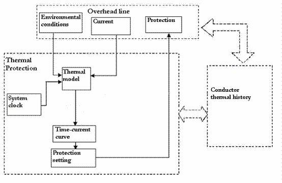
The choice of temperature alarm shall be determined by two principles:
¸ must not be too close to the max. conductor temperature to allow longer time for action;
¸ must not be too far from the max. conductor temperature not to lose the advantage of knowing only the lines at increased risk of overload, and then use the best processing capacity of the system.
In the diagram there is also a block that return in real time the remaining life of the conductor, calculated from the knowledge of the "history" heat of the latter; this information will be very useful for further analysis of the conductor line (i.e. it is possible to determine the maximum time for which a specific over temperature can remain without risk of excessive deterioration of the conductor).
Conclusions
In many Countries the demand for electric power is constantly increasing, and there is a corresponding requirement to increase the power transferred by transmission and distribution lines. A solution would be to build or re-conduct new lines but this may not be feasible on account of economic or environmental considerations.
The analysis of the influence of the ambient conditions justifies the use of a dynamic thermal rating of the line that permits to satisfy new requirements of network thank to these advantages:
¸ increase of the transferred power;
¸ real-time monitoring to determine the rating of the line;
¸ possibility to use self-adaptive protection device;
¸ update the rest-life of conductor;
¸ flexibility of the electric system.
References
1. Piegari L., Rizzo R., Tricoli P., A Comparison between Line-Start Synchronous Machines and Induction Machines in Distributed Generation, Prezglad Elektrotechniczny (Electrical Review), ISSN 0033-2097, 2012, 88(5b), p. 187-193.
2. Rizzo R., Tricoli P., Spina I., An innovative reconfigurable integrated converter topology suitable for distributed generation, Energies, ISSN 1996-1073, 2012, 5(9), p. 3640-3654.
3. Brando G., Dannier A., Del Pizzo A., Rizzo R., Power Electronic Transformer for Advanced Grid Management in Presence of Distributed Generation, International Review of Electrical Engineering IREE, ISSN 1827-6660, 2011, 6(7), p. 3009-3015.
4. Andreotti A., Del Pizzo A., Rizzo R., Tricoli P., An efficient architecture of a PV plant for ancillary service supplying, International Symposium on Power Electronics Electrical Drives Automation and Motion SPEEDAM, Pisa , 2010, p. 678-682.
5. CIGRE WG B2.12, Conductors for the uprating of overhead lines, ELECTRA, ISSN: 1286-1146, 2004, 213, p. 30-39.
6. Carlini E.M., Favuzza S., Giangreco S.E., Massaro F., Quaciari C., Uprating an Overhead Line, Italian TSO Applications for Integration of RES, Proceedings of ICCEP, Alghero (Italy), ISBN 978-1-4673-4430-2, 2013.
7. Douglass D.A., Edris A., Real time monitoring and dynamic thermal rating of power transmission circuits, IEEE Trans. on Power Delivery, 1996, 11, p. 1407-1418.
8. Douglass D.A., Lawry D. C., Edris A., Bascom E. C., Dynamic thermal ratings Realize circuit load limits, IEEE Computer Application in Power, 2000, 13, p. 38-44.
9. Adapa R., Douglass D.A., Dynamic thermal ratings: monitors and calculation methods, IEEE Power Engineering Society Inaugural Conference and Exposition in Africa, 2005.
10. Musavi M., Chamberlain D., Qi L., Overhead conductor dynamic thermal rating measurement and prediction, IEEE International conference on Smart Measurement for future grids, 2011, p. 135-138.
11. Douglass D.A., Weather-dependent versus static thermal line ratings, IEEE Transaction on power delivery, 1988, 3, p. 742-753.
12. Marzorati A., Elisei G., Zanzottera E., Galletti E., Misura di parametri meteorologici mediante sistemi di telerilevamento attivo, L’Elettrotecnica, 1992, 7(8), p. 798-801.
13. Bonelli P., Di Sabato E., Uso dei filtri adattativi per la previsione della temperatura dell'aria, L'energia elettrica, 1994, 71, p. 412-419.
14. Hall J.F., Deb A.K., Prediction of overhead transmission line ampacity by stocastic and deterministic models, IEEE Transaction on power delivery, 1988, 3, p. 789-800.
15. Morgan V.T., The radial temperature distribution and effective radial thermal conductivity in bare solid and stranded conductors, IEEE Transaction on Power Delivery, 1990, 5, p. 1443-1452.
16. CIGRE WG 22.12, Thermal behaviour of overhead conductors, Techinical Brochure 2002, 207, p. 1-46.
17. IEEE STD 738-2006, IEEE Standard for Calculating the current-temperature of bare overhead conductors, IEEE Power engineering society, 2007, p. 1-59.
18. Black W.Z., Rehberg R.L., Simplified model for steady state and real time ampacity of overhead conductors, IEEE Transaction on power apparatus and systems, 1985, vol.PAS-104, p. 2942-2953.
19. Black W.Z., Byrd W.R., Real time ampacity model for overhead lines, IEEE Transactions on Power Apparatus and Systems, 1983, vol. PAS-102, p.2289-2293.