Adaptive wavelet neural network for wind speed and solar power forecasting for Italian data

D. Rakesh CHANDRA¹, Francesco GRIMACCIA², Sonia LEVA³, Marco MUSSETTA⁴,
M. Sailaja KUMARI⁵, Sydulu M.⁶, Zich RICCARDO⁷

¹ Politecnico di Milano - Dept. of Energy Via La Masa 34, 20156 Milano, Italy

² National Institute of Technology, Warangal, India

E-mails: rksh.chndr@gmail.com; francesco.grimaccia@polimi.it; sonia.leva@polimi.it; marco.mussetta@polimi.it

^*Corresponding author, Phone: +39 389 0432170;

Fax: +39 02 2399 8566

Abstract

Conventional energy sources are nowadays exhausting and that is the reason why renewable energy sources are so important in current situation. In addition renewables are non-pollutant and freely available in nature. Wind and solar power are the fastest growing renewable energy sources for the past few decades, especially according to the 2020 energy strategy in Europe. They are having enough scope in the power market. The main problem with these renewable energy sources is their unpredictability and, in this context, issues like power quality and power system grid stability arise. In order to limit the effects of these issues, power market needs information about power generation at least one day in advance. This problem can be addressed by proper forecasting of Renewable Energy Sources (RES). Forecasting helps to schedule power properly. Adaptive Wavelet Neural Network (AWNN), a technique already assessed in literature for wind speed forecasting, is here applied also to solar power prediction. After forecasting each individual signal, the Mean Absolute Percentage Error (MAPE) is calculated in different time horizons.

Keywords

Forecasting; Renewables; Morlet wavelet; Adaptive wavelet neural network

Introduction

In recent days the significance of renewable energy sources has been increasing. Renewable energy is the best alternative for the conventional energy sources.  Renewable energy sources are abundant in nature, whereas conventional energy sources are exhausting day by day [1]. In this context, a growing interest is now devoted to the development of smart systems, in order to suitably manage the electrical energy distribution among different areas, optimizing the mix of both renewables and traditional sources [2].

With the emergence of renewables into the power system, forecast of power generation by renewables gained much more importance for proper grid operation. Many different tools and techniques have been developed to handle wind forecasting problem. A Wind speed forecasting can be done by Ensemble Empirical Mode Decomposition (EEMD) [3] and in combination with support vector machine (SVM). In this method decomposed wind data by EEMD can be forecasted individually by using SVM. Neural networks are often used for wind speed forecasting and for that neural networks can be trained by Back propagation algorithm (BPA) [4, 5]. In [6] Adaptive Neuro Fuzzy Inference Systems [ANFIS] is used for wind speed forecasting for power generation in countries like Tasmania, Australia. Hybrid methods are also used for wind speed forecasting [7]. Hybrid methods are combination of Wavelet transform (WT), Particle Swarm Optimization (PSO), ANFIS. In [8] many wind speed forecasting methods have been discussed. In [9] two statistical model based wind speed forecasting methods namely Autoregressive Moving Average (ARMA) and Neural networks (NN) based forecasting methods have been discussed. Novel approaches like empirical mode decomposition (EMD) and time series analysis [10] are used for wind speed prediction for a practical data in North china. Wavelets are also used for wind speed forecasting [11, 12]. Here wind speed series is decomposed and each decomposed signal is forecasted individually. Later all these signals are then combined to get final forecasted signal. Wavelets have been also used for energy price forecasting [13]. Data mining algorithms are also useful to predict wind speed and wind power [15]. In [16], 48 hours ahead forecasting has been done by using a statistical method. In [17] an evolutionary optimization algorithm tool has been introduced to train artificial neural network for energy forecasting of PV plants. In [18, 19] the role of computational tools is discussed and issues related to PV plants in connection with smart grid are highlighted. Exogenous (ARX) based spatio temporal model has been proposed in [20] for solar power forecast. This ARX model outperforms other models and results in a more accurate forecast. In [21] a novel integrated wind and solar power forecasting is proposed. In [22] artificial neural network and generalizing neural networks have been used for renewable energy forecasting. A hybrid intelligent algorithm which uses a combination of a data filtering technique based on wavelet transform has been used in [23] for short term forecasting of PV generated power. In future renewables will increase their share in power generation [24].

Here we will employ Adaptive Wavelet Neural Network (AWNN) for forecasting application in wind power generation, which is a well-assessed application in literature [12]; moreover, we will apply the same technique to solar power prediction, to explore AWNN performance in this new application field. In the coming sections AWNN model, implementation and results are presented, followed by their discussion and conclusion.

Material and method

In this paper wavelets are used for wind speed and solar power forecasting. A Morlet wavelet eight level decomposition is used for wind speed forecasting and Morlet seven level decomposition is used for solar power forecasting. Number of decomposition levels is based on number of samples available for forecasting. The considered wind plant in this paper (wind speed) is located in Abruzzo region, near Isernia, Central Italy. The PV data under analysis refer to a plant located Lazio region, near Viterbo, Central Italy, and 132 m above sea level. Number of wind samples used are 8760 and solar samples are 7081. Wind samples represent hourly based wind speed and solar samples represent 15mins based solar power. This paper aims regarding accuracy in forecasting where APE (Absolute Percentage Error) there by MAPE (Mean Absolute Percentage Error) is minimized.

Adaptive wavelet neural network (AWNN)

A wavelet is a tiny wave which can increase and decrease the amplitude and width of the wave in a fixed time period. Wavelet properties make them more suitable to solve many problems in engineering applications. In wavelets translation, dilation parameters (generally represented as a, b) which reflect length, breadth of a wavelet. These parameters will adjust according to the problem type, and varied accordingly. They are easily adaptable, flexible and they can fit too many complex problems. Compared to neural networks wavelets training is accurate since wavelets consist of translation, dilation parameters. Wavelet analysis is also advantageous if compared to Fourier series analysis. In Fourier analysis in fact every signal can be expressed either in sine or cosine waveforms, while in wavelet analysis a suitable wavelet can be chosen from a family of wavelets. Fourier analysis is suitable to analyse either frequency or time but not both at a time, whereas in wavelet analysis that is possible. In other words wavelets can be better suited for time varying frequency analysis. Wavelet satisfies below two fundamental properties by which it can be said that wavelets are also like ordinary waves [12, 14].

	(1)
	(2)

Several types of wavelets exist in literature. Depending on type of the problem suitable wavelet type can be chosen. Here in this paper, Morlet wavelet has been used for wind speed and solar power forecasting. A Complete one year (2011) of Wind speed data has been collected from an Italian wind farm and 7081 samples of PV data has been collected from another PV plant. A wavelet multi resolution analysis (MRA) technique has been used, which decompose wind and PV signal to obtain approximate and detailed coefficients. Decomposition makes signal easier to be predicted and by that noise can be eliminated so resulting in a more accurate prediction. Generally approximate coefficients (represented by S) are used to analyse low frequency signals and detailed coefficients (represented by D) are used to analyse high frequency signals. Finally these two coefficients combination is used to analyse signal at all levels so that signal can be analysed accurately. Each of these coefficients are forecasted for next 24 hours ahead in the case of wind and for 3, 6, 9, 12 hours ahead in case of PV, after that all  these forecasted signals are added to reconstruct original signal by using Wavelet Methods for Time series Analysis (WMTSA) in MATLAB. In this paper back propagation algorithm was used to train the network. Wavelet networks are the combination of wavelet decomposition and neural networks. Wavelet neural networks are similar to feed forward networks except that input layer is connected to hidden layer as well as output layer.

Morlet mother wavelet

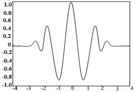
Here in this paper Morlet mother wavelet has been chosen for forecasting. Morlet wavelets (Figure 1) are generally used for signals with rapid variations. Wind speed variations and solar power variations (especially with high variable weather conditions) are drastic so Morlet wavelet is a suitable solution for this forecasting application. Figure 2 shows wavelet neural network where u₁,u₂ …u₅₀ shows input wind velocities in case of wind speed prediction and solar power inputs in case of solar power prediction. z₁, z₂, z₃ are hidden nodes, v₁, v₂,… v₅₀ are weights connected between input to output and w₁,w₂……w_m are weights connected between hidden to output node[12]. Where “m” denotes number of weights and here m=3. In Wavelet neural network, hidden layer consists of wavelet function.

Parameters used to train AWNN Network:

¸ Learning rate (η) = 0.5,

¸ Momentum coefficient (α) = 0.5,

¸ Tolerance (ε) = 0.0001,

¸ Number of input nodes = 50,

¸ Number of hidden nodes = 3.

As anticipated in this work, Morlet wavelet is being used as a mother wavelet. The following equations explain forecasting processor by using AWNN.

Figure 1. Morlet wavelet (from [14])

Figure 2. Wavelet neural network (from [12])

            Morlet mother wavelet is defined as:

(3)

where  is represented as wavelet function.

            The translation and dilation version of Morlet wavelet is represented by

(4)

where.

            The output  for the hidden layer neurons is represented as

(5)

            The output of the WNN, which is represented as a decomposed signal of the hour ahead forecast can be calculated as

(6)

where  indicates the weight from the ^th wavelon to output node, and denotes the weight from the th input node to output node, and  is known to be bias at output node.

Mean square error (E) is given by 

and

(7)

where  is the model output and  is the desired output for a given ^th input pattern. The free parameter is updated by following formula 

(8)

            where

(9)

and Г represents an unknown free variable, η is a learning rate and α represent momentum parameter. The change in free parameters by using (20) is

	(10)
	(11)

Figure 3. Decomposition of Wind Signal up to Eight Levels by using MRA

Figure 4. Decomposition of PV Signal up to Seven Levels by using MRA

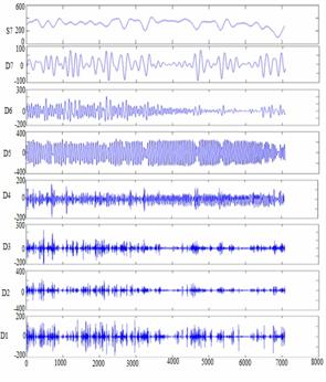
Decomposition of wind and PV signals has been shown in Figures 3 and 4 respectively. Similar algorithm is used to forecast the wind signal using Morlet wavelet as a mother wavelet neural network [25].

Implementation

The standard Back Propagation gradient descent Algorithm (BPA) has been used in this article for training the Wavelet Neural Network (WNN). BPA is a supervised learning that is output is known for every individual forecasting which is here called to be as target. Error will be calculated based on difference between output (target) and forecasted value. Based on this error weights will be adjusted. Due to particular properties of WNN (Wavelet Neural Network) it becomes flexible, suitable, and adjustable to new purposes or conditions. Particular properties which make WNN to AWNN are hidden layer consists of wavelet function and additional direct connection between input and output.

The algorithm for Wind Speed and solar power forecasting using AWNN Network follows these rules

1. From 1 to 50 wind samples from input to AWNN and target is 51^st sample.

2. From 2 to 51 wind samples are input to AWNN and target is 52^nd sample.

3. Similarly proceed for next 60 patterns that is last pattern is from 60^th to 109^th wind sample. These 60 patterns are used to train the network.

4. This process is adopted for D₁ to Dn and Sn.  Here “n” denotes the level of decomposition.

5. Finally the problem is converged for different iterations from D₁ to Dn and Sn. Where D and S denotes detailed and approximating coefficients respectively.

6. After the problem is converged, final weights, translation and dilation parameters are used to predict 24 hours ahead samples in the case of wind and 3, 6, 9, 12 hours in the case of PV.

7. Forecasting has been done from 2554 to 2577 in the case of wind, and from the same sample to 3, 6, 9, 12 hours ahead in case of PV by taking inputs from 2504 to 2553 and output has taken recursively at every instant. Same procedure has adapted from D₁ to Dn and Sn.

8. Finally all these coefficients (from D₁ to Dn and Sn) are added to get the original forecasted wind speed.

            Decomposition results of wind signal and solar signals are shown in Figures 3 and 4.

Results and discussions

Here actual values of wind speed are measured through one anemometer located in the plant site, 1400 m AMSL (above mean sea level). Global irradiation (PV) is measured on a horizontal plane by a first class pyranometer (uncertainty of 5%, confidence level 95%) and by a secondary standard pyranometer (uncertainty of 2%).

Table 1 shows comparison of actual wind speed and predicted wind speed for 24 hours ahead. Table 2, 3, 4, and 5 shows the comparison of actual and predicted solar power for 12 (3 hours), 24 (6 hours), 36 (9 hours), 48 (12 hours) samples respectively. In all these cases Absolute Percentage Error (APE) has been calculated and average of all APEs give Mean Absolute Percentage Error (MAPE) and all these analysis have been shown in the graphs below from figures 4 to 9. APE is calculated as

·

·

where w_m and w_p are wind speed actual and predicted values, respectively, while p_m and p_p are solar power actual and predicted values, respectively. Tables 2 to 5 represent solar power forecast for different samples 12, 24, 36, 48 which is equivalent to 3, 6, 9, 12 hours respectively as every solar sample is 15 mins average solar power. Here figures 5 to 9 are graphical representations to tables 1 to 5.

Table 1. Comparison of actual and forecasted wind speed for Morlet wavelet with eight levels decomposition

S.No	Actual wind speed in m/s	Forecasted wind speed in m/s	APEwind
1	2.133334	2.3628967	10.7607482
2	3.283332	3.120539	4.95816445
3	2.900001	2.694639	7.081445834
4	2.949999	3.196636	8.360579105
5	2.566667	2.480044	3.37492164
6	1.683334	1.706261	1.361999461
7	2.916667	3.0668	5.147416555
8	2.416666	2.229105	7.761146969
9	2.166666	2.154931	0.541615551
10	2.516668	2.302144	8.524127934
11	1.200001	1.303184	8.598576168
12	1.116666	1.114681	0.1777613
13	0.783333	0.782517	0.104170257
14	2.566667	2.504663	2.415739946
15	3.099999	2.759943	10.96955193
16	4.499999	4.138978	8.022690672
17	4.833332	4.584005	5.158491078
18	6.033331	4.916358	18.5133718
19	5.766666	4.539897	21.27345333
20	5.833332	5.127283	12.10369991
21	6.8	5.853006	13.92638235
22	6.299997	5.555933	11.81054531
23	5.399999	5.615309	3.987222961
24	3.849999	4.691636	21.86070698
MAPE:			8.199

Figure 5. Actual and forecasted wind speed time series using Morlet wavelet as a base wavelet for eight levels of decomposition

Table 2. Comparison of actual and forecasted solar power for Morlet wavelet with seven level decomposition up to 12 samples

S.No	Actual solar power in watts	Forecasted solar power in watts	APEsolar
1	37.878788	56.430795	48.97729832
2	65.454545	64.35897	1.673795151
3	96.969699	98.755693	1.841806274
4	120.606061	117.760726	2.359197354
5	152.424242	148.890373	2.318442889
6	190.303031	191.333739	0.541614074
7	195.454547	200.337684	2.498349143
8	256.96966	229.440907	10.71284174
9	289.090871	238.440221	17.5206674
10	329.999962	261.101466	20.87833453
11	368.78784	271.203599	26.46080766
12	409.393902	293.885673	28.21444785
MAPE			13.66

Figure 6. Actual and forecasted PV power using Morlet Wavelet as a base wavelet for seven levels of decomposition up to 12 samples

Table 3. Comparison of actual and forecasted solar power for Morlet wavelet with seven levels decomposition up to 24 samples

S.No	Actual solar power in watts	Forecasted solar power in watts	APEsolar
1	37.878788	51.160005	35.06241277
2	65.454545	59.692791	8.802679783
3	96.969699	94.54704	2.498367041
4	120.606061	129.781329	7.607634247
5	152.424242	169.781845	11.38769186
6	190.303031	208.509633	9.567163436
7	195.454547	243.42424	24.54263343
8	256.96966	293.737212	14.30812961
9	289.090871	305.078707	5.530384251
10	329.999962	329.953914	0.013953941
11	368.78784	345.524576	6.308034451
12	409.393902	364.696611	10.91791812
13	444.848447	361.34326	18.77160358
14	484.545416	334.289539	31.00965813
15	520.302954	345.006161	33.69129305
16	536.96962	441.161226	17.84242356
17	560.302953	572.264036	2.134752804
18	590.909015	663.067248	12.21139485
19	613.636288	685.761219	11.75369391
20	639.999924	658.860016	2.946889725
21	656.060531	619.166515	5.623568902
22	668.787803	596.325688	10.83484398
23	675.15144	602.262843	10.79588855
24	684.84841	605.968236	11.51790277
MAPE			12.736

Figure 7. Actual and forecasted PV power using Morlet Wavelet as a base wavelet for seven levels of decomposition up to 24 samples

Table 4. Comparison of actual and forecasted solar power for Morlet wavelet with seven levels decomposition up to 36 samples

S.No	Actual solar power in watts	Forecasted solar power in watts	APEsolar
1	37.878788	35.151541	7.199932057
2	65.454545	44.641267	31.79806383
3	96.969699	83.914836	13.46282719
4	120.606061	109.262972	9.405073763
5	152.424242	148.32308	2.690623188
6	190.303031	187.698107	1.368829485
7	195.454547	199.452462	2.045444868
8	256.96966	219.425363	14.6104007
9	289.090871	204.357961	29.31012996
10	329.999962	222.825199	32.47720465
11	368.78784	237.559776	35.58362011
12	409.393902	270.94006	33.8192243
13	444.848447	343.141637	22.86324942
14	484.545416	393.082063	18.87611563
15	520.302954	469.149558	9.83146369
16	536.96962	516.268355	3.855202274
17	560.302953	546.547114	2.455071658
18	590.909015	570.976903	3.373127079
19	613.636288	590.21342	3.817060441
20	639.999924	613.187075	4.189508154
21	656.060531	638.166794	2.727452141
22	668.787803	663.949867	0.723388791
23	675.15144	670.723002	0.65591773
24	684.84841	672.535627	1.79788444
25	693.333258	665.392975	4.029848947
26	702.727196	661.135009	5.918681849
27	674.242348	635.075215	5.809058585
28	579.696894	605.240964	4.406452797
29	701.515075	607.08047	13.46152184
30	685.7575	557.6966	18.67437104
31	680.605985	604.99367	11.10955776
32	674.242348	622.381249	7.691759373
33	679.696895	614.029521	9.661273206
34	635.151439	607.160954	4.406899407
35	660.909015	641.616174	2.919137213
36	450.606022	547.450268	21.49199994
MAPE			11.069

Figure 8. Actual and forecasted PV power using Morlet Wavelet as a base wavelet for seven levels of decomposition up to 36 samples

Table 5. Comparison of Actual and Forecasted solar power for Morlet wavelet with Seven Level Decomposition up to 48 samples

S.No	Actual solar power in watts	Forecasted solar power in watts	APEsolar
1	37.878788	41.159952	8.662272932
2	65.454545	56.134417	14.23908454
3	96.969699	87.926054	9.326258711
4	120.606061	116.824825	3.135195668
5	152.424242	151.668784	0.49562851
6	190.303031	190.612963	0.162862356
7	195.454547	216.198651	10.61326243
8	256.96966	247.973868	3.500721447
9	289.090871	262.270009	9.277657889
10	329.999962	288.00037	12.72715056
11	368.78784	304.701453	17.37757595
12	409.393902	334.102472	18.39095053
13	444.848447	399.397508	10.21717381
14	484.545416	435.476463	10.12680161
15	520.302954	499.163173	4.062975395
16	536.96962	528.449439	1.586715651
17	560.302953	536.630807	4.22488332
18	590.909015	543.723507	7.985240841
19	613.636288	557.772769	9.1036857
20	639.999924	582.407455	8.99882435
21	656.060531	614.875428	6.277637665
22	668.787803	643.331558	3.806326145
23	675.15144	660.151131	2.221769534
24	684.84841	673.025606	1.726338826
25	693.333258	680.791222	1.808947697
26	702.727196	677.63296	3.570978346
27	674.242348	665.752154	1.259219927
28	579.696894	654.094879	12.83394577
29	701.515075	636.041201	9.333209839
30	685.7575	629.505939	8.202835696
31	680.605985	661.688418	2.779518167
32	674.242348	663.107411	1.651473989
33	679.696895	666.860829	1.888498549
34	635.151439	668.189452	5.201596182
35	660.909015	651.641114	1.402296048
36	450.606022	563.21685	24.99097271
37	211.21212	461.921397	118.7002323
38	319.99996	371.264963	16.02031544
39	509.999925	324.16545	36.43813771
40	472.727233	248.340361	47.46645768
41	240.909091	261.834877	8.686175317
42	247.272728	278.220327	12.51557309
43	198.787878	173.021386	12.96180243
44	100.606061	159.109852	58.1513583
45	53.939393	95.732739	77.4820473
46	71.212121	79.596111	11.77326259
47	104.848485	100.996507	3.673851844
48	99.69697	112.766056	13.10880963
MAPE			13.961

Figure 9. Actual and forecasted PV power using Morlet Wavelet as a base wavelet for seven levels of decomposition up to 48 samples

Here the wind speed and solar power forecasted results have been analyzed. In Adaptive Wavelet Neural Network (AWNN) a Morlet mother wavelet is used for both wind speed and solar power forecasting. Here for both wind and solar forecasting, selfsame Adaptive Wavelet Neural Network (AWNN) with Morlet mother wavelet is used. Here real production of wind and solar data is used for forecasting.

Table 1 represents the actual and forecasted wind speed for 24 hours ahead. This wind data has been provided by Italian wind farm where some part of data is not accurate for forecasting due to malfunction of anemometers or recording errors. And here forecasted samples are taken from 2554 to 2577 where values are good enough for forecasting application.

Conclusions

In this paper wind speed and solar power have been forecasted using AWNN. Wind speed has been forecasted for 24 hours ahead and solar power is forecasted in 3, 6, 9, 12 hours ahead. Here for both wind and solar their Mean Absolute Percentage Error (MAPE) has been compared. Here for wind speed forecasting hourly wind data and for solar 15 minutes average solar power have been taken. For wind speed Forecasting MAPE is 8.199 and in the case of solar it varies from 11.069 to 13.961. In case of solar among all MAPE’s 36 samples (9 hours) gives the best MAPE as 11.069 after that 24 sample (6 hours). In case of 12 samples (3hours), 48 samples (12 hours) give errors as 13.66, 13.961 respectively. These excess errors in 12, 48 samples are due to involvement of extreme (low) values of a particular day. Forecasting of extreme values is not much accurate as they involve a low value which leads to higher values of error. In case of PV 48 samples (equivalent to 12 hours) is the maximum because solar power is available only in day time. Forecasting results are good in case of PV, but significantly more accurate in case of wind as Morlet wavelet is more accurately adaptable for problems with sudden variations. In future AWNN model has to be developed such that even hours including extreme values (sun rise, sun set hours) in a day are also more accurately predicted.

References

1. Kaplan O., Yavanoglu U., Issi F., Country study on renewable energy sources in Turkey, International Conference on renewable energy research and applications (ICRERA), 2012, p.1-5.

2. Marmiroli M., Tsukamoto Y., Mitsubishi electric smart grid for a future low carbon society, Innovative smart grid technologies (ISGT), 2012.

3. Song J., A new method for the short-term wind speed forecasting, 4th International Conference on electric utility deregulation and restructuring and power technologies (DRPT), 2011, p. 1320 – 1324.

4. Wu L., Park J., Choi J., Cha J., Lee K.Y., A study on wind speed prediction using artificial neural network at Jeju Island in Korea, Transmission & Distribution Conference & Exposition, 2009, p.1-4.

5. Barbounis T., Theocharis J., Alexiadis M., and Dokopoulos P., Long term wind speed and power forecasting using local recurrent neural network models, IEEE Trans. eergy convers., 2006, 21(1), p. 273–284.

6. Potter C.W., Negnevitsky M., Very short-term wind forecasting for Tasmanian power generation, IEEE Transactions on power systems, 2006, 21(2), p. 965 – 972.

7. Catalao J.P.S., Pousinho H.M.I., Mendes V.M.F, Hybrid wavelet-PSO-ANFIS approach for short-term wind power forecasting in Portugal, IEEE Transactions on sustainable energy, 2011, 2(1), p.50 – 59.

8. Rakesh Chandra D., Sailaja Kumari M., Sydulu M., A detailed literature review on wind forecasting, International conference on power, energy and control (ICPEC), 2013, p. 630 – 634.

9. Gomes P., Castro R., Comparison of statistical wind speed forecasting models, World Congress on sustainable technologies (WCST), 2011, p. 56 – 61.

10. Liu X.-J., Mi Z.-Q., Lu B., Tao W., A novel approach for wind speed forecasting based on EMD and time-series analysis, Power and energy engineering conference, 2009, p.1-4.

11. Khan A.A., Shahidehpour M., One day ahead wind speed forecasting using wavelets, Power systems conference and exposition, 2009, p.1-5.

12. Bhaskar K., Singh S.N., AWNN-Assisted wind power forecasting using feed-forward neural network, IEEE Transactions on sustainable energy, 2012, 3(2), p.306-315.

13. Pindoriya N.M., Singh S.N., Singh S.K., An adaptive wavelet neural network-based energy price forecasting in electricity markets, IEEE Transactions On power systems, 2008, 23(3), p.1423-1432.

14. Moraud E.M., Wavelet networks, A report, 2009.

15. Kusiak A., Zheng H., and Song Z., Short-term prediction of wind farm power: A data mining approach, IEEE Transactions on energy conversion, 2009, 24(1), p. 125-136.

16. Sideratos G., Hatziargyriou N.D., An advanced statistical method for wind power forecasting, IEEE Transactions on power systems, 2007, 22(1), p. 258-265.

17. Grimaccia F., Mussetta M., Zich R., Neuro-fuzzy predictive model for fuzzy PV energy production based on weather forecast, Fuzzy systems (FUZZ), 2011 IEEE International conference on digital object identifier, 2011, p. 2454 – 2457.

18. Grimaccia F., Mussetta M., Zich R.E., Adavanced predictive models towards PV energy integration in smart grid, IEEE International conference on fuzzy systems (FUZZ_IEEE), 2012, p. 1-6.

19. Caputo D., Grimaccia F., Mussetta M., Zich R.E., Photovoltaic plants predictive model by means of ANN trained by a hybrid evolutionary algorithm, The 2010 International joint conference on neural networks (IJCNN), p.1-6.

20. Yang C., LeXie, A novel ARX – based multi-scale spatio temporal solar power forecast moddel, North american power symposium (NAPS), 2012, p. 1-6.

21. Zhongping Y., Weimin L., Feng G., Tao W., Gaili Z., Bin W., Xiaoguang R., Haifeng W., Integrated wind and solar power forecasting in China, Service operations and logistics, and informatics (SOLI), 2013 IEEE International Conference on, 2013, 505(28-30), p.500.

22. Singh V.P., Vaibhav K., Chaturvedi D.K., Solar power forecasting modeling using soft computing approach," Engineering (NUiCONE), 2012 Nirma University International Conference, p.1,5, 6-8 Dec. 2012.

23. Ashraf Haque U., Hashem Nehrir M., Mandal P., Solar PV power generation forecast using a hybrid intelligent approach, Power and energy society general meeting (PES), 2013 IEEE, p.1,5, 21-25 July 2013.

24. Rizzo R., Direct current smart micro-grids for distributed generation with renewable energy sources, Leonardo electronic journal of practices and technologies, 2013, 12(12), p.27-42.

25. Rakesh Chandra D., Sailaja Kumari M., Sydulu M., Comparison of ANN, AWNN for wind speed forecasting Studies, International electrical engineering journal, 5(2), p.2078-2365.