Optimization of partially shaded PV array using a modified P&O MPPT algorithm

Abdelaziz YOUCEF¹, Abdallah MILOUDI¹, Rafik SAYAH², Houari SAYAH²

¹ Electrical Engineering Department. Genie Electrical Laboratory (LGE), Moulay Tahar University, Saida, 20000, Algeria

²Electrical Engineering Department. Intelligent Control and Electrical Power System Laboratory (ICEPS), Djillali Liabes, University, Sidi-Bel-Abbes, 22000, Algeria

E-mails: youcefazziz@yahoo.fr, amiloudidz@yahoo.fr, Rafik_vrai@hotmail.fr,

housayah@yahoo.fr

^* Corresponding author, phone: 00213 775196954, fax: 0021348473979

Received: February 11, 2016 / Accepted: July 17, 2016 / Published: July 31, 2016

Abstract

A photovoltaic (PV) array generated power is directly affected by temperature, solar irradiation, shading, and array configuration. In practice, PV arrays could be partially shaded by could, buildings, trees and other utilities. In this case, multiple maximums appear in the P-V curve, a global maximum and one or several local maximums. The “perturb and observe“ (P&O) maximum power point tracking (MPPT) algorithm cannot differentiate between a global and a local maximum and it is therefore ineffective when partial shading occurs. First, this paper presents an original mathematical model of the P-V curve of a partially shaded PV array, that was used to perform a simulation study in order to show the P&O algorithm inability to track the global MPP of a PV array solar system under partial shading for low shading irradiation levels, then an adaptation sub algorithm is proposed to be added to the P&O algorithm in order to give it the ability to track the global MPP. This sub algorithm moves the operating point imposed by the partial shading configuration to a point in the vicinity of the global MPP in order to be easily tracked by the P&O algorithm. In the simulation, a PV array with a hundred modules has been considered by using a light, a medium then a severe shading configuration. The results obtained indicate that the proposed modified P&O algorithm is able to track the global MPP for the considered shading configurations and for any shading irradiation level.

Keywords

Maximum Power Point tracking (MPPT); Perturb and Observe (P&O); Photovoltaic array (PV); Shading; Uniform irradiation

Introduction

Nowadays, renewable energy is gradually beginning to play an important role in the production of electricity. Among these new energies (biomass, wind, solar, geothermal), photovoltaic (PV) solar energy represents the best option for the future since it is unlimited, available everywhere, can be used freely and emits almost no pollution during use.

PV solar energy is produced from solar radiation using solar modules consisting of PV cells in series. However, despite the technological advances in the field of cells manufacturing, the efficiency of such a system is still low and its short term energy production cost remains still higher than ordinary power plant. To overcome this problem, research has been directed towards performance optimization of a PV solar system by extracting its maximum power for any driven load. Indeed, because of the I-V characteristics of the solar PV system, the power generated by the system varies with the driven load.

A result of these researches was the MPPT (Maximum Power Point Tracker) method which allows the control of the static converter between the load and the PV solar system in order to continuously provide the maximum power to the load. Maximum power point tracker (MPPT) uses a high efficiency DC to DC converter that converts the power to a voltage level which is more suitable to whatever load the system is designed to drive. PV cells have a single operating point where the values of the current (I) and Voltage (V) result in a maximum power output. Maximum power point trackers use an algorithm to search for this point and thus to allow the converter circuit to extract the maximum power available from a cell.

Several MPPT algorithms have been proposed by researchers [1-9], the most used are: Perturb & Observe, Incremental Conductance, and Constant Voltage. These methods are based on finding the maximum of the P-V curve of the PV solar system and are effective only when the curve has only one maximum. However, in the case of partial shading of the PV solar system, several local maximum can appear along with the global maximum in the P-V curve making the maximum power point tracking with conventional MPPT methods ineffective [10-15].

In this paper we are going to study the impact of partial shading on the power delivered by a PV array solar system when the P&O MPPT tracking algorithm is used. Then an adaptation sub algorithm is proposed to be added to the P&O algorithm in order to give it the ability to track the global MPP. A PV solar system of 10 series assemblies of ten modules each arranged in parallel is subjected to chosen shading patterns with a grid of irradiation levels in order to investigate the global MPP tracking ability of the proposed method.

Material and method

Modeling and simulation of a PV array under uniform irradiation

As represented by Figure 1, the equivalent circuit of a one diode PV cell is composed of a diode, a current source, a series resistance, and a parallel resistance [16-20]. The light generated current (I_L) is a function of the incident solar irradiation and the cell temperature. The PV cell p–n junction is represented by the diode. The series resistance (R_S) is used to take into account the observed voltage loss on the way to the external contacts of the PV cell. Furthermore, a shunt resistance (R_P) is used to express the leakage currents.

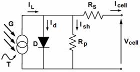
Figure 1. Equivalent circuit of a PV cell

Using Kirchhoff’s first law, the equation for the I–V curve is derived as follows:

(1)

where:

	(2)
	(3)
	(4)
	(5)

I_cell and V_cell are the PV cell output current and voltage respectively, V_t is the thermal voltage, I₀ is the diode reverse bias saturation current, q is the elementary charge (1.6´10^-19  C), k is the Boltzman constant (1.38·10^-23 J/K), T  is the cell temperature (K) and n is the diode ideality factor of the PV cell. Thus, the I-V characteristics of the PV cell are given by:

(6)

A PV module composed of N_S solar cells in series, have the same output current as the solar cell and an output voltage given by:

(7)

The I-V characteristic of the PV module is then given by:

(8)

From equation (8) at V=0, an expression of the PV module short circuit current I_SC is obtained as:

(9)

For an ideal solar cell (R_S → 0, R_P → ∞) we can write:

(10)

Then equation (8) becomes:

(11)

The instantaneous value of the short circuit current can be found by using the following equation [15]:

(12)

where I_sc,stc is the standard condition short circuit current of the PV module which is  provided by the PV module manufacturer, G and G_stc are respectively the instantaneous and standard condition solar irradiance on the PV module, T and T_stc are respectively the instantaneous and standard condition temperature of the PV module and α is the short-circuit current temperature coefficient of a PV cell. Since G_stc = 1000 W/m² and the temperature variation effect on the value of I_sc is negligible (less than 1%), we can write (where V_oc is the PV module open circuit voltage):

	(13)
	(14)

On the other hand, PV module in series-parallel connection can form a PV array. The PV array voltage V_A, current I_A and power P_A under uniform irradiation can be obtained from the module voltage V and current I as:

(15)

where N_ss and N_pp are respectively the series and parallel number of PV modules in the array.            A Matlab program has been written in order to solve equations (11) and (15) and plot I-V and P-V curves of the PV array under uniform irradiation. The diode ideality factor n was taken as unity. The PV module manufacturer datasheet used in this paper is given by table 1.

Table 1. PV module manufacturer’s data

Open circuit voltage  Voc	21.9V
Short-circuit current Isc	4.95 A
Optimal voltage Vm	17.5 V
Optimal current Im	4.57 A
Maximal Power Pm	80 W
Series resistance RS at Tstc	0.0102 Ω
Shunt resistance RP at Tstc	4.6278 Ω

The solution of equation (11) is obtained, for a grid of values of the current I, by using the bisection method to solve the equation  in the interval  where is given by:

(16)

The Matlab program was executed for a (10x10) PV array ( and ). Figure 2 shows the resulting P-V curve of the PV array. The P-V curve has the form of a hill with one maximum operating point.

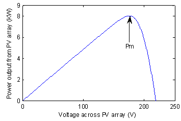
Figure 2. Output P-V characteristic of the PV array under uniform irradiation illumination shading of 100 W/m²

Modelling and simulation of a PV array with partial shading

To model a PV array with partial shading we need first to model the shading pattern on that array. The special categorization and terminology given by Patel [14] is used for this purpose. Figure 3 shows a PV array solar system of 100 modules divided into ten series assemblies of 10 modules each, connected in parallel.

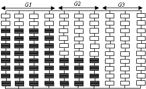
Figure 3. PV array solar system of 10 series assemblies connected in parallel, divided into groups with the same shading pattern

When subjected to partial shading, these series assemblies are assembled into groups having the same shading pattern. The shading configuration of Figure 3 gives three groups (G₁ to G₃).The series assemblies of G₁ have eight shaded modules each, those of G₂ have four shaded modules each whereas the series assemblies of G₃ have no shaded module.

Let us consider a group of N_cg columns with N_ss modules in series, having similar shading configuration with N_sm shaded modules under an irradiation level equal to G (kW/m²). The irradiation of the unshaded modules is equal to 1 kW/m². For a grid of values of the voltage V_A, across a column, the corresponding values of the current I flowing in the column are calculated using the following method. From Figure 3, the PV Array column voltage is given by:

(17)

where V₁ and V₂ are the voltages across the shaded and unshaded modules respectively.

Using equation (11) we can define the function:

(18)

            Because V₁ is the voltage across a module with current I and subjected to a shading irradiation level G≤1, V₁ is then the solution of the equation f(V, I, G) = 0. On the other hand V₂ is the solution of the equation f(V, I, 1) = 0. We can symbolize this by the following equations:

	(19)
	(20)

The column current value I is that which allows the voltages V₁ and V₂ given by equations (19) and (20) to satisfy equation (17). Using equations (17-20), we can define the function g(I) given by:

(21)

The value of the column current I is then the solution of equation  which could be obtained by the bisection method.

Results and discussion

Applying this model, a Matlab program was developed to plot the P-V curve of a partially shaded PV array. This program has been executed for the PV array of Figure 4 where all the unshaded modules receive an irradiation level of G = 1 kW/m².

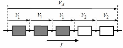
Figure 4. PV Array column voltage diagram

Figure 5 shows the effect of partial shading on the characteristics of the PV array.

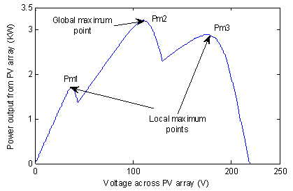
Figure 5. P-V curve of the partially shaded PV array given by Figure 3 when the shaded module irradiation level is 0.1 kW/m²

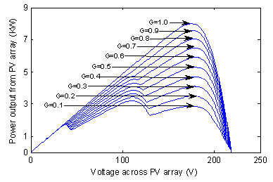
Figure 6. P-V curves of the partially shaded PV array given by fig. 3 for different irradiation levels

It gives the P-V characteristic of the array when the shaded modules receive an irradiation level of G = 0.1 kW/m². We can see from this figure that the P-V curve is formed of three different hills with three maximum power points, two local maximums and one global maximum.

Figure 6 shows the P-V curves of this array as the irradiation changes in steps of 0.1 kW/m². It is clear from the figure that the power increases with the increase of the shaded module irradiation level. Furthermore, the variation of the shaded modules irradiation level changes the position of the global MPP.

Partial shading effect on the P&O MPPT controlled PV array

To maximize the output power of a PV array solar system, continuous maximum power point tracking of the system is necessary (Figure 7).

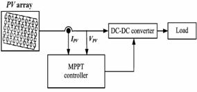
Figure 7. Block diagram of an MPPT controlled PV array solar system

Let us consider the general case when the PV array of Figure 3 was under full irradiation before being subjected to the given shading configuration. If the P&O MPPT algorithm is applied to track the MPP, then before shading occurs, the tracked maximum power is P_m = 8 kW. When the given shading configuration is applied, the position of the maximum available power point changes but the voltage used by the MPPT algorithm is still around V_m. The P&O MPPT algorithm continues the tracking process and tracks the summit of the hill that includes the operating point with voltage V_m. It has no way to know if the tracked MPP, is global or local. In this section we are going to study the effect of partial shading on the P&O MPPT algorithm by studying the power loss caused by the inability of the P&O MPPT algorithm to track the global MPP when partial shading occurs. A simulation study was done in order to obtain the position of the three different MPPs along with the tracked MPP for different shading levels under the shading pattern given by Figure 3.

Table 2 gives the position of the maximum points of the P-V characteristics for a grid of values of G.

Table 2. MPPs position for different shading irradiation level G with the shading configuration of Figure 3

G(W/m²)	50	100	200	300	400	500	600	700	800	900	1000
Pm1(W)	1707	1707	1707	1707	1707	1707	1707	1707	1707	-------	-------
Pm2(W)	3099	3208	3426	3645	3865	4086	4307	4530	4725	-------	-------
Pm3(W)	2587	2886	3488	4093	4698	5300	5896	6480	7045	7570	7997

Table 3 shows the effect of partial shading on the P&O MPPT algorithm for a grid of values of G. It gives the P&O tracked power and the maximum available power.

From Table 3 we can see that the P&O algorithm is not able to track the maximum power point for low shading irradiation levels (< 200 W/m²). The P&O algorithm is unable to differentiate between global peaks and local peaks. For low shading irradiation levels the MPPT algorithm is trapped around one of the local peaks resulting in significant power loss. There is up to 16% power loss for G=50W/m².

Table 3. P&O algorithm Power tracking loss for different shading irradiation levels with the shading configuration of Figure 3

G (W/m²)	50	100	200	300	400	500	600	700	800	900	1000
Maximum Power (W)	3099	3208	3488	4093	4698	5300	5896	6480	7045	7570	7997
Tracked Power (W)	2587	2886	3488	4093	4698	5300	5896	6480	7045	7570	7997
Power Loss (%)	512	322	0	0	0	0	0	0	0	0	0

Figure 8 shows that for a sudden change in the shading irradiation level (from 1000 to 100 W/m²), the MPP tracked value using the P&O algorithm converges to 2886 W and not towards the global MPP who is 3208 W. The P&O algorithm is not able to differentiate between the local and global peak for low irradiation values.

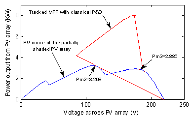
Figure 8. P&O tracking process from a uniform standard irradiation to the partial shading configuration of Figure 3 with shading level of 0.1 kW/m²

P&O adaptation algorithm to track the partially shaded PV array global MPP

In this section we are going to propose an adaptation of the P&O algorithm in order to give it the ability to track the global MPP of a partially shaded PV array. When the PV array is under uniform irradiation, the unique MPP of the P-V characteristic could be easily tracked by the P&O algorithm. If partial shading occurs, the power delivered by the PV array will drop significantly and several local MPP’s might arise in the P-V characteristic. In this case, the P&O algorithm is no longer able to track the global MPP unless the operating point at that instant is on the hill of the global MPP. Our proposition is to add a sub algorithm to the P&O algorithm in order to shift the operating point to a point on the hill of the global MPP.

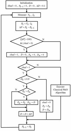
Figure 9. Flowchart of the modified P&O algorithm

The proposed sub algorithm, which is executed whenever a significant power drop is observed, performs a rapid span along the whole voltage interval in order to search for the operating point that delivers the maximum power. When this point is attained, the P&O algorithm could be used to successfully track the global MPP. The span algorithm we propose to use is executed for a very short time only when a significant power drop is observed. In our study the power drop is interpreted as a partial shading problem but this is not the only interpretation of power drop. Nevertheless our proposition can be used to track the global MPP when any PV array default that can cause power drop occurs.

Figure 9 gives the flowchart of the proposed modified P&O algorithm for global MPP tracking. In this algorithm the occurrence of partial shading is interpreted by a power variation of ±100W. The solution we propose in order to solve the global MPP tracking problem is to do a span of the duty cycle D while saving the maximum value of the power obtained in the process. This will detect the true global MPP.

A Matlab program was developed in order to simulate the implementation of the proposed method to the MPPT controlled PV array solar system of Figure 7 under partial shading. To test our improved MPPT algorithm, the search for global MPP was simulated using a (10x10) GPV. The GPV is uniformly isolated at first, before the shading configuration of figure 03 occurs at t=2s with a shading level of G=100W/m². Figures 10 and 11 show the simulation results.

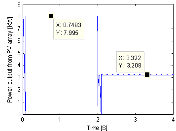
Figure 10. Curve of P(t) with variation of G for configuration of Figure 4

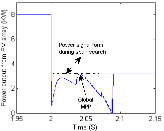
Figure 11. Zoom of P(t) in the vicinity of t= 2s

When shading occurs the generated power is seen to move along the PV characteristic of the  partially shaded GPV during a span search period of less than 0.1 s before it settles at the global MPP, namely: P=3208 W. To strengthen this result, and compare it to that of the classical P&O algorithm, a set of simulations using the modified and classical P&O algorithms respectively, were performed on a (10x10) GPV that starts with (a) a uniform irradiation before it is subjected to (b) a light shading configuration at t=1s followed by (c) a medium shading configuration at t=2s and finally by (d) a severe shading configuration at t=3s, as shown in Figure 12.

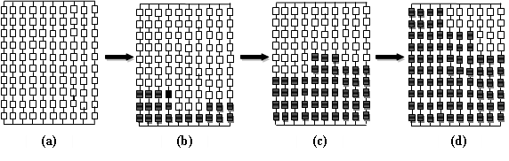
Figure 12. Different configurations with: (a) Uniform irradiation, (b) light shading,

(c) average shading, (d) severe shading

These four different configurations allow us to know whether the modified algorithm has the capacity to follow the global MPP for low irradiation levels. Figure 13 and 14 give the simulation results for an irradiation levels G=100W/m² and 150W/m² respectively.

Modified P&O

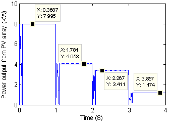
Classical P&O

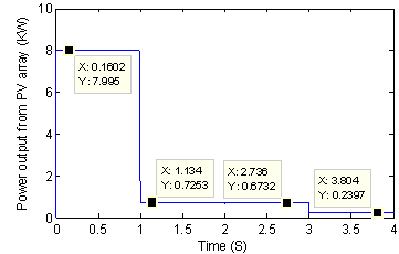
Figure 13. Generated power with the modified and classical P&O algorithm for the configurations of Figure 12 with G=100W/m²

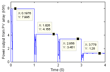
Modified P&O

Classical P&O

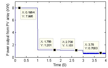
Figure 14. Generated power with the modified and classical P&O algorithm for the configurations of figure 10 with G=150W/m²

We can say from these figures that the modified P&O algorithm allows the GPV to generate the global maximum power for any shading configuration and any irradiation level. Table 4 gives a comparison between the classical and modified P&O algorithm for each shading configuration and for G= 100W/m² and 150W/m².

Table 4. Generated power using modified end classical P&O algorithm for Figure 10 shading configurations and for G=100 and 150 W/m².

G = 100 W/m²

G = 150 W/m²

Configuration		(a)	(b)	(c)	(d)
Generated Power (W)	Classical P&O	7995	725	673	240
	Modified P&O	7995	4053	3411	1174
	Power gain (%)	0.0	459	407	389

Configuration		(a)	(b)	(c)	(d)
Generated Power (W)	Classical P&O	7995	1201	1151	700
	Modified P&O	7995	4155	3451	1280
	Power gain (%)	0.0	247	200	83

As we can see from these figures, the proposed span algorithm was able to move the operating point imposed by the shading configurations to the neighborhood of the global MPP, making it easy to be tracked by the P&O algorithm. The proposed span algorithm resulted in a rapid P&O global MPP tracking.

It increases the power generated by the classical P&O algorithm from around 460% for the light shading configuration to around  390% for the severe configuration when G=100 W/m². It increases the power generated by the classical P&O algorithm from around 250% for the light shading configuration to around 90% for the severe configuration when G=150 W/m².

From these results we can say that the proposed modification of the P&O algorithm allowed the tracking algorithm to follow rapidly the global MPP and solved the low irradiation MPP tracking problem of the classical P&O algorithm.

Conclusions

In this paper we first presented an original mathematical model of the P-V curve of a partially shaded PV array that was used to perform a simulation study of the P&O maximum power point tracking algorithm applied to a partially shaded (10x10) PV array.

This study showed the inability of the P&O algorithm to track the PV array global MPP for low shading irradiation level, causing up to 16% power for a 50 W/m² shading irradiation level.

We then proposed to add an adaptation sub algorithm to the P&O algorithm that moves the operating point imposed by the partial shading configuration to a point in the vicinity of the global MPP in order to be easily tracked by the P&O algorithm.

The simulation result of the modified P&O MPPT algorithm used on a partially shaded (10x10) PV array showed a perfect ability of the proposed algorithm to track the global MPP for any shading configuration and any shading irradiation level.

The added adaptation algorithm resulted in an increase of the PV array generated power of around 460% for a light shading configuration and with a shading irradiation level of 100W/m².

Finally, these results lead us to say that the proposed P&O adaptation method can solve the global MPP tracking problem of the classical P&O algorithm.

Appendix

PV	Photovoltaic
P&O	Perturb and observe
MPPT	maximum power point tracking
MPP	maximum power point
Q	elementary charge (=1.6´10^-^19 C)
K	Boltzman  constant  (=1.38´10^-23J/°K)
N	diode ideality factor of the PV cell
I0	diode reverse bias saturation current
RS, RP	series and parallel resistance in the equivalent circuit of the model respectively
IL	light generated current
Icell, Vcell	PV cell output current and voltage respectively
Ish	current through the shunt resistance
T, Tstc	instantaneous and standard condition temperature of the PV module respectively
a	short-circuit current temperature coefficient of a PV cell
Vt	thermal voltage
Isc, Voc	short circuit current and open circuit voltage of the PV the module respectively
Ns	solar cells in series
Nss, Npp	series and parallel number of PV modules  in the array respectively
Isc, stc	standard condition short circuit current of the PV module
G, Gstc	instantaneous and standard condition solar irradiance on the PV module respectively
Ncg	number of columns per group
Nsm	number of shaded modules

References

1. Brambilla A., Gambarara M., Garutti A., Ronchi F., New approach to photovoltaic arrays maximum power point tracking, Conf. Rec. PESC’99, Charleston, South Carolina, 1999, p. 632–637.

2. Kim T. Y., Ahn H. G., Park S. K., Lee Y. K., A novel maximum power point tracking control for photovoltaic power system under rapidly changing solar radiation, in IEEE Int. Symp. Ind. Electron., 2001, p. 1011-1014.

3. Liu X., Lopes L. A. C., An improved perturbation and observation maximum power point tracking algorithm for PV arrays, Conf. Rec. PESC’04, Aachen, Germany, 2004, p. 2005-2010.

4. Liu C., Wu B., Cheung R., Advanced Algorithm for MPPT Control of Photovoltaic Systems,Conf. Rec. of the first Canadian Solar Buildings Conference, Montreal, 2004.

5. Femia G., Petrone G., Spagnuolo G., Vitelli M., Optimization of perturb and observe maximum power point tracking method, IEEE Trans. Power Electron., 2005, 20(4), p. 963-973.

6. Xiao W., Lind J., Dunford W., Capel A., Real-Time Identification of Optimal Operating Points in Photovoltaic Power Systems, IEEE Transactions on Industrial Electronics, 2006, 53(4), p. 1017-1026.

7. Hernandez J. C., Jurado F., Photovoltaic Devices under Partial Shading Conditions, International Review on Modelling and Simulations (IREMOS), 2012, 5(1), p. 414-425.

8. Ramaprabha R., Mathur B. L., Comparative Study of Series and Parallel configurations of Solar PV Array under Partial Shaded Conditions, International Review on Modelling and Simulations, 2014, 3(6), p. 1363-1371.

9. Mostefai M., Miloudi A., Miloud Y., An Intelligent Maximum Power Point Tracker for Photovoltaic Systems Based on Neural Network, International Review on Modelling and Simulations, 2013, 51, p. 29-38.

10. Hussein K. H., Muta I., Maximum photovoltaic power tracking: An algorithm for rapidly changing atmospheric conditions, Proc. Inst. Electr. Eng. Gener., Transmiss. Distrib., 1995, 142(1), p. 59-64.

11. Koutroulis E., Kalaitzakis K., Voulgaris N. C., Development of a microcontroller-based photovoltaic maximum power point tracking control system, IEEE Trans. Power Electron., 2001, 16(1), p. 46-54.

12. Jain S., Agarwal V., A new algorithm for rapid tracking of approxi-mate maximum power point in photovoltaics systems, IEEE Power Electron. Lett., 2004, 2(1), p. 16-19.

13. Hecktheuer L.A., Krenzinger A., Prieb C. W. M., Methodology for Photovoltaic Modules Characterization and Shading Effects Analysis, Journal of the Brazilian Society of Mechanical Sciences, 2002, 24(1), p. 26-32.

14. Patel H., Agarwal V., Matlab-Based Modeling to Study the Effects of Partial Shading on PV Array Characteristics, IEEE Trans. on Energy Conversion, 2008, 23(1), p. 302-310.

15. Parlak K. S., Can H., A new MPPT method for PV array system under partially shaded conditions, Conf. Rec. PEDG 2012, Aalborg, Denmark, 2012, p. 437-441.

16. Teng K. F., Wu P., PV module characterization using Q-R decomposition based on the least square method, IEEE Transactions on Industrial Electronics, 1989, 36(1), p. 71-75.

17. Duffie J. A., Beckman W. A., Solar Engineering and Thermal Processes., John Wiley & Sons Inc., New York, 1991.

18. Merten J., Asensi J. M., Voz C., Shah A. V., Platz R., Andreu J., Improved  equivalent circuit and analytical model for amorphous silicon solar cells and modules, IEEE Transactions on Electron Devices, 1998, 45(2), p. 423-429.

19. Ikegami T., Maezono T., Nakanishi F., Yamagata Y., Ebihara K., Estimation of equivalent circuit parameters of PV module and its application to optimal operation of PV system, Solar Energy Materials and Solar Cells, 2001, 67, p. 389-395.

20. Araki K., Yamaguchi M., Novel equivalent circuit model and statistical analysis in parameters identification, Solar Energy Materials and Solar Cells, 2003, 75(3), p. 457-466.