Engineering, Environment

An accurate estimation and optimization of bottom hole back pressure in managed pressure drilling

Boniface Aleruchi ORIJI, Nsikak Maurice MARCUS^*

Department of Petroleum Engineering, University of Port Harcourt, Nigeria.

E-mail(s): aloriji2000@yahoo.com; marcus.nsikak@yahoo.com;

^*Nsikak Maurice Marcus, phone: +2348035098606,

Received: November 24, 2016 / Accepted: June 16, 2017 / Published: June 30, 2017

Abstract

Managed Pressure Drilling (MPD) utilizes a method of applying back pressure to compensate for wellbore pressure losses during drilling. Using a single rheological (Annular Frictional Pressure Losses, AFPL) model to estimate the backpressure in MPD operations for all sections of the well may not yield the best result. Each section of the hole was therefore treated independently in this study as data from a case study well were used. As the backpressure is a function of hydrostatic pressure, pore pressure and AFPL, three AFPL models (Bingham plastic, Power law and Herschel Bulkley models) were utilized in estimating the backpressure. The estimated backpressure values were compared to the actual field backpressure values in order to obtain the optimum backpressure at the various well depths. The backpressure values estimated by utilizing the power law AFPL model gave the best result for the 12 1/4" hole section (average error % of 1.855%) while the back pressures estimated by utilizing the Herschel Bulkley AFPL model gave the best result for the 8 1/2" hole section (average error % of 12.3%). The study showed that for hole sections of turbulent annular flow, the power law AFPL model fits best for estimating the required backpressure while for hole sections of laminar annular flow, the Herschel Bulkley AFPL model fits best for estimating the required backpressure.

Keywords

Managed Pressure Drilling; Back Pressure; Annular Frictional Pressure losses; Bingham Plastic model; Power Law model; Herschel Bulkley model; Hydrostatic pressure; Pore Pressure

Introduction

The world's population continues to grow at a geometric rate, which means there will be a proportionate increase in demand of energy. For this reason, engineers and scientists are in constant search of newer sources of energy and new ways to completely exploit existing energy sources. Today, there is a constant decline in crude reserves hence the need to explore more challenging and complex environments. Drilling in these challenging environments using the conventional drilling method could easily lead to drilling hazards such as: Kick; lost circulation; borehole instability and stuck pipe which are the major contributors to Non-Productive Time (NPT) [1]. Discoveries have shown that NPT account for approximately 20% of total rig time and can be much higher in difficult and complex terrains. Rig rates are on the high, with some rigs going for as high as $1M per day, showing the strong impact of NPT on drilling cost. As the challenge of a narrow drilling window becomes increasingly pronounced, drilling with the conventional method will lead to the setting of many casing strings at relatively shallower depth as a result of trying to avoid the obvious drilling problems. This also leads to a reduced productivity and a higher well cost. MPD is now seen as a technology that may provide a noteworthy increase in cost-effective drill-ability by reducing excessive drilling related costs typically related to conventional offshore drilling, knowing that about 70% of current crude oil offshore reserves cannot be drilled economically using the conventional method of drilling [2]. MPD is very effective in reducing NPT that are drilling related and also enable the drilling of prospects that technically and economically are not feasible to drill using the normal conventional drilling method.

According to the International Association of Drilling Contractors (IADC), Managed Pressure Drilling is an adaptive drilling process that is used to precisely control the annular pressure profile throughout the wellbore [3]. MPD is therefore an advanced form of well control where a closed and pressurized mud system is applied to enable a more precise control of wellbore pressure profiles than just mud hydrostatic and the pump pressure adjustments [3]. The primary objective of MPD is to get the pressure limits of the down hole and proportionally manage the hydraulic annular pressure profile. MPD may include control of backpressure, fluid density, fluid rheology, annular fluid level, circulating friction, and hole geometry or combinations thereof. MPD has been proven to enable drilling of what might otherwise be economically un-drillable prospects and MPD is good on its way to becoming the status quo technology over the next decade due to the fact that it increases recoverable assets [3]. The Constant Bottom Hole Pressure (CBHP) variation of MPD is a technique associated with the control of backpressure to attain the goal of an MPD operation. The required back pressure term for MPD operation is very important to achieve a successful CBHP MPD operation. Therefore, it is necessary to have a very reliable tool for estimating the required back pressure. Another challenge with the CBHP MPD operation is that most of the methods used in the hydraulics calculations in MPD operations assume just one rheological model in all hole sections, meanwhile in reality, different sections of the hole may fit best to different rheological models.

A simulated research was carried out to determine the best rheological model in predicting pressure losses in drilled wells [4]. The Bingham Plastic, Power law and Herschel Bulkley models were all compared. The pressure losses gotten from these three models were compared to the pressure losses gotten from field data of wells drilled with both water and oil base mud. It was found that no one model was completely adequate, as rheological behaviour changed from one hole section to another. On the whole though, it was concluded that the Herschel Bulkley model was best in predicting pressure losses in the pipe (96% accuracy) while the power law model was best in predicting annular pressure losses (93%) [4]. Use of MPD technologies can influence many wellbore pressure-related drilling challenges, including lost circulation, kicks, wellbore ballooning, tight pore pressure(PP)/fracture pressure (FP) margins, close tolerance casing programs, wellbore stability problems, shallow water/gas flows, slow ROP, etc [5]. These technologies may also enable future well programs that are currently thought to be conventionally “undesignable” with single gradient mud systems [5]. Some experimental analysis were carried out in [6] to ascertain the best fluid rheology model for HPHT condition (40 to 2800F and 500 to 12000psi) using un-weighted n-paraffin base drilling fluid (synthetic mud) in MPD operations. An equation to model the effect of temperature and pressure on drilling fluid density was developed. They compared the Bingham plastic, Power law and Yield power law models to their experimental findings. The yield power law gave the most accurate result when compared to the experimental result [6]. Hence the Yield power law at the actual hole temperature and pressure was used as the yardstick to check for the accuracy in using Bingham Plastic and Power law models to estimate the pressure gradients with surface parameters using different flow rates. From the study it was found that the discrepancies between pressure gradients gotten at actual well temperature and surface condition increased as the flow rate decreased and it was concluded that the Bingham plastic model with surface parameters would estimate pressure gradients with the least error at low temperature conditions while the power law model with high shear rate parameters would estimate both pipe and annuli pressure gradient with the highest accuracy [6]. In [7] it was stated that drilling-grade barite limits drilling fluids design for wells with critically narrow hydraulic operating windows. This limitation can be overcome by formulating a Treated Micronized Barite (TMB) instead of API barite, as TMB produces a low rheology fluid that may reduce the downhole frictional pressure by 0.5ppg with minimal risk of barite sag or settlement [7]. A new approach to drilling fluid design that uncoupled fluid rheology from the risk of barite sag and settlement was developed. This was accomplished by reducing the particle size of API barite from 97% less than 75 microns to 97% less than 5 microns, hence the rate of sedimentation in the drilling fluid was significantly reduced [7]. A study to know how pressure control is affected and sometimes limited by the actual available data and its quality, equipment, hydraulic models, control algorithm and down hole condition during MPD operations in ERD wells was carried out in [8]. In planning MPD in long wells, it is very vital to establish the limits on what can be accurately and robustly achieved [8]. It was concluded that special care should be taken when applying MPD in ERD wells because, ERD wells are more complex and challenging when compared to shorter wells [8]. In [9] a careful study of the Herschel Buckley model was carried out and a new model was developed by modifying the Herschel Buckley model. An explicit equation between the wall shear stress and the volumetric flow rate for pipe and annular flow from Herschel Buckley fluid model was developed [9]. A new relation for pipe and annular Reynolds number and frictional pressure drop was established. The new model was validated using well data from Sichuan Basin and it was concluded that the new model predicted and calculated hydraulics more accurately than the other traditional models previously used in MPD operations [9]. Simulation analysis for kick detection, control and circulation using MPD were carried out in [10]. The benefits of automated influx detection and control using MPD system compared to a conventional well control method were highlighted. The simulations successfully detected and controlled a gas influx in oil based mud while drilling in onshore western Canada. It was concluded that the current MPD system has the potential for drilling formations with narrow pressure margins through their accuracy and precision in pressure control and early kick detection [10]. In [11] a simple hydraulics model called the "fit-for purpose" hydraulics model was developed and it was used for computing the downhole pressures and to provide a choke pressure set point for automated MPD systems. In [12] a successful application of MPD in a deep exploration well offshore Egypt was described. It was concluded that utilizing the CBHP technique of MPD could minimize the problems in the wells.

The use of MPD is becoming more popular especially in offshore application to mitigate drilling hazards and enhance production rates which in turn maximizes profit. The main aim of this study is to apply the concepts of Constant Bottom Hole Pressure (CBHP) technique of MPD to develop a computer model (using visual basic dot net) that can estimate and optimize the backpressure required to mitigate drilling hazards during MPD operations. This study also aims to propose the best rheological (AFPL) model that will give a perfect fit for the drilling hydraulics calculation for CBHP MPD operations for the various hole sections of well.

Material and Method

The importance of mitigating drilling hazards cannot be overemphasized. The problems of lost circulation, borehole instability, kick and stuck pipe remains the major cause of NPT and should be properly managed and controlled. The ability to precisely control the pressures in the wellbore will go a long way in helping to minimize these problems.

Data Collection from the field

The data used for this study were obtained from a field in West Africa and it included the pore pressure, fracture gradient, rheological properties of the fluid used, hole size and depth, drill string components, sizes and lengths. The well comprised of three hole sections. The 17 1/2" hole, 12 1/4" hole and the 8 1/2" hole sections. The 17 1/2" hole section was drilled using the conventional drilling technique. But the 12 1/4" and 8 1/2" hole sections were drilled using Managed Pressure Drilling (MPD) techniques as shown in tables 3 and 4 of the appendix.

Analysis Method

A software model (Marc.soft) was developed using visual basic.Net programming language, to estimate the backpressure from the pore pressure, hydrostatic pressure and manipulation of the AFPL models. The MarcSoft computer software is user friendly and easy to manipulate. Data can either be typed directly into software or uploaded from an excel file into the software. The software also evaluated the percentage errors from using each of the three stated AFPL models (Bingham plastic, power law and herschel bulkley) respectively for backpressure estimation. This approach made it easy to select the most accurate AFPL model for MPD operations in the various well sections/depths as the estimated back pressure values were compared to the actual backpressure values from the field data.

For MPD operations, the Bottom Hole Pressure (BHP) must be maintained in between the Pore Pressure (PP) and Fracture Pressure (FP) for effective control. In the CBHP method of MPD, the BHP is a function of the mud hydrostatic pressure (HP), the annular friction pressure losses (AFPL) and the Back pressure (BP), Eq. (1).

BHP = HP + AFPL + BP (1)

But, Eq. (2):

PP ≤ BHP ≤ FP (2)

Combining equations 1 and 2, Eq. (3):

BP ≥ PP - (AFPL + HP) (3)

Where: MW - mud weight, ppg; TVD - true vertical depth, ft.

HP = 0.052 x MW x TVD; (4)

Three AFPL models (Bingham plastic, power law and Herschel bulkley) were utilized for this study so as obtain the best model for optimal backpressure estimation.

Bingham Plastic model

The constitutive Bingham Plastic fluid equation is given as Eq. (5-7):

(5)

Where: τ - shear stress; τ_y - yield point (lb/100ft²); µ_p - plastic viscosity (cp); γ - shear rate (sec^-1).

μ_p = ϴ₆₀₀ - ϴ₃₀₀ (6)

τ_y = ϴ₃₀₀ - µ_p (7)

Where: ϴ₆₀₀ - dial reading at 600 viscometer RPM, ϴ₃₀₀ - dial reading at 300 viscometer RPM

If flow is laminar (eq. 8),

(8)

Where: µ_p - plastic viscosity (cp); v = average velocity (ft/sec); d₂- hole or casing diameter (inches); d₁ - drill string diameter (inches); τ_y - yield point (lb/100ft²); AFPL - annular frictional pressure losses (psi).

If flow is turbulent (Eq. 9):

(9)

Turbulent criteria, Eq. (10 and 11):

(10)

(11)

For Bingham plastic fluid, flow is turbulent if N_Re> 2100 (Bourgoyne et al 1991)

Where: N_Re - Reynolds number; µ_a - apparent viscosity (cp); µ_p - plastic viscosity (cp); ρ - fluid density (ppg); L - length/depth (ft); AFPL - annular frictional pressure losses (psi); v - average velocity (ft/sec); d₂ - hole or casing diameter (inches); d₁ - drill string diameter (inches); τ_y - yield point (lb/100ft²).

Power law model

Power law model is represented by Eq. (12-17):

τ = Kγⁿ (12)

Where: K = Consistency Index, n = flow behavior index, γ = shear rate (sec^-1),

(13)

(14)

Where: ϴ₁₀₀ - dial reading at 100 viscometer RPM; ϴ₃ - dial reading at 3 viscometer RPM; K_a - consistency index (in annulus); n_a = flow behavior index (in annulus).

(15)

(16)

Where: f - friction factor; AFPL - annular frictional pressure losses (psi); ρ - fluid density (ppg), L - length/depth (ft); v - average velocity (ft/sec); d₂ - hole or casing diameter (inches); d₁ - drill string diameter (inches); µ_a - apparent viscosity (cp).

(17)

If flow is laminar, Eq. (18):

(18)

If flow is turbulent, Eq. (19-21):

(19)

Where: f - friction factor; Ka - consistency index (in annulus); na - flow behavior index (in annulus), all other reoccurring parameters remain the same.

(20)

(21)

Turbulence criteria:

- If N_Re is less than 3470 - 1370n, the flow is laminar;

- If N_Re is greater than 4270 - 1370n, flow is turbulent;

- But if N_Re is between (3470 - 1370n) and (4270 - 1370n) flow is transitional and we have Eq. (22):

(22)

Where: N_Re, n, a and f are the same as in preceding equations.

Herschel Bulkley model

The Herschel Bulkley model is given by the equations 23-28:

(23)

Where: K = consistency index; n - flow behavior index; γ - shear rate (sec^-1); τ_y - yield point (lb/100ft²); τ = shear stress (psi).

(24)

(25)

(26)

Where: ϴ₆₀₀ - dial reading at 600 viscometer RPM, ϴ₃₀₀ - dial reading at 300 viscometer RPM; NRe - Reynolds number; v - average velocity (ft/sec); ρ - fluid density (ppg); d₂ - hole or casing diameter (inches); d₁ - drill string diameter (inches); τ_y - yield point (lb/100ft²); L - length/depth (ft).

(27)

Where: K - consistency Index, n - flow behavior index, d₂ - hole or casing diameter, (inches), d₁ - drill string diameter (inches), τ_y - yield point (lb/100ft²), Q - pump rate (GPM).

(28)

Where: f - friction factor; AFPL - annular frictional pressure losses (psi); ρ - fluid density (ppg); d₂ - hole or casing diameter (inches); d₁ - drill string diameter (inches); L - length/depth (ft); Q - pump rate (GPM).

Turbulence criteria, Eq. 23-33:

(29)

(30)

(31)

If N_Re is less than Nre_cr, the flow is laminar,

If N_Re is greater than Nre_cr, the flow is turbulent.

If flow is laminar, Eq. (32):

(32)

If flow is turbulent, Eq. (33):

(33)

Figure 1 is a flow chat that was developed to depict the mode of operation of the Marc.Soft software application for estimation and optimization of backpressure for MPD operations.

The first thing to do after entering the Marc.Soft environment is to input data. The data can be manually entered into the software by selecting the 'sample data' option otherwise select the 'import data' option to directly upload the data from an existing MS Excel file. The next step is to select the Annular Frictional Pressure Loss (AFPL) models one after the other until all three AFPL models programmed (Bingham plastic, Power law and Herschel Bulkley AFPL models) have all been selected. The next step is to select the “evaluate back pressure” option to effect the estimation of back pressure using all three AFPL models at once. Next step is to validate the back-pressure estimates from all three models by confirming the percentage error estimates gotten from using each of the three AFPL models as compared to the actual field back pressure. Select the AFPL model with the least error and then end.

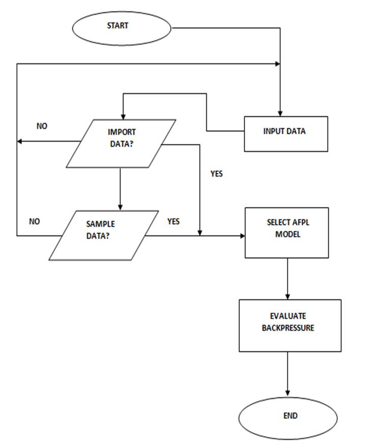
Figure 1. Flow Chart for Back Pressure Estimation from Marc.Soft (2016)

The following assumptions were made during developing this optimization model:

1. The drill string is concentrically placed in the open hole.

2. The open hole sections are circular in shape with known diameters.

3. The drilling fluid is incompressible.

4 Temperature and pressure have opposing effects on the fluid rheology, hence their overall effect on the drilling fluid is neutral.

Results and discussion

The summary of the results gotten from utilizing the three rheological models are presented here. The focus was to get the AFPL model that gave the best estimate of the back pressure to enable proper design and a real-time analysis for an MPD system. The well data as shown in tables 3 and 4 in the appendix were for the two different hole sections (12.25" and 8.5''). MPD was used in this well because of the narrow drilling window between the pore pressure and the fracture gradient. The results were presented according to individual hole sections. The well data in the Appendix (table 3) were obtained from a field in West Africa.

Results for the 12 1/4" hole section

The estimated Back pressure values from the different AFPL models for this hole section are shown below in table 1 (table 1 is an extract from the developed software).

Table 1 - The estimated back pressures from using each of the three AFPL models and their respective error % estimate (3930 to 8300 ft)

Depth	Field Back Pressure, Psi	Bingham Plastic, BP* (psi)	Power law BP* (psi)	Herschel Bulkley BP* (psi)	Error % from Bingham Plastic BP*	Error % from power law BP*	Error % from Herschel Bulkley BP*
3930.00	449.30	425.98	453.78	452.91	-5.19	1.00	0.80
3980.00	443.32	382.82	447.62	434.15	-13.65	0.97	-2.07
4000.00	444.49	384.75	449.87	436.33	-13.44	1.21	-1.83
4100.00	454.55	394.37	461.12	447.24	-13.24	1.44	-1.61
4200.00	465.55	403.99	472.36	458.15	-13.22	1.46	-1.59
4300.00	476.33	413.60	483.61	469.06	-13.17	1.53	-1.53
4400.00	487.80	423.22	494.86	479.97	-13.24	1.45	-1.61
4500.00	498.97	432.84	506.10	490.88	-13.25	1.43	-1.62
4600.00	510.16	442.46	517.35	501.78	-13.27	1.41	-1.64
4700.00	521.11	452.08	528.60	512.69	-13.25	1.44	-1.62
4800.00	532.53	461.70	539.84	523.60	-13.30	1.37	-1.68
4900.00	543.44	471.32	551.09	534.51	-13.27	1.41	-1.64
5000.00	554.68	480.94	562.34	545.42	-13.29	1.38	-1.67
5200.00	577.44	500.17	584.83	567.23	-13.38	1.28	-1.77
5400.00	600.18	519.41	607.32	589.05	-13.46	1.19	-1.85
5600.00	621.61	538.65	629.82	610.87	-13.35	1.32	-1.73
5800.00	643.69	557.89	652.31	632.68	-13.33	1.34	-1.71
6000.00	665.93	577.12	674.80	654.50	-13.34	1.33	-1.72
6300.00	699.72	605.98	708.54	687.23	-13.39	1.26	-1.79
6600.00	731.12	634.83	742.28	719.95	-13.17	1.53	-1.53
6900.00	764.47	663.69	776.02	752.68	-13.18	1.51	-1.54
7000.00	775.71	673.31	787.27	763.58	-13.20	1.49	-1.56
7100.00	787.17	682.93	798.52	774.49	-13.24	1.44	-1.61
7200.00	798.07	692.55	809.76	785.40	-13.22	1.47	-1.59
7300.00	809.08	702.17	821.01	796.31	-13.21	1.47	-1.58
7400.00	820.11	711.78	832.26	807.22	-13.21	1.48	-1.57
7500.00	831.00	721.40	843.50	818.13	-13.19	1.50	-1.55
7600.00	842.23	731.02	854.75	829.03	-13.20	1.49	-1.57
7700.00	479.26	428.17	488.84	451.12	-10.66	2.00	-5.87
7800.00	482.69	433.73	495.19	456.98	-10.14	2.59	-5.33
7900.00	486.94	439.29	501.53	462.83	-9.79	3.00	-4.95
8000.00	493.80	444.85	507.88	468.69	-9.91	2.85	-5.08
8020.00	881.43	757.51	897.18	864.74	-14.06	1.79	-1.89
8040.00	881.20	759.40	899.41	866.89	-13.82	2.07	-1.62
8060.00	892.50	770.86	904.97	876.08	-13.63	1.40	-1.84
8080.00	894.18	772.78	907.22	878.26	-13.58	1.46	-1.78
8100.00	898.76	775.03	909.53	881.35	-13.77	1.20	-1.94
8120.00	900.53	776.94	911.78	883.52	-13.72	1.25	-1.89
8140.00	901.78	778.85	914.02	885.70	-13.63	1.36	-1.78
8160.00	857.53	699.04	887.59	819.91	-18.48	3.51	-4.39
8170.00	857.83	699.89	888.68	820.91	-18.41	3.60	-4.30
8180.00	856.97	700.75	889.77	821.92	-18.23	3.83	-4.09
8190.00	858.94	701.61	890.85	822.92	-18.32	3.72	-4.19
8200.00	859.75	702.46	891.94	823.93	-18.29	3.74	-4.17
8300.00	511.32	467.60	520.46	476.70	-8.55	1.79	-6.77
BP*: Back Pressure

Results for the 8 1/2" hole section

The estimated Back pressure values from the different AFPL models for this hole section are shown below in table 2 (table 2 is an extract from the developed software).

Table 2 - The estimated back pressures from using each of the three AFPL models and their respective error % estimate (8300 to 13500 ft)

Depth	Field back pressure (psi)	Bingham plastic, BP* (psi)	Power law BP* (psi)	Herschel Bulkley BP* (psi)	Error % from Bingham Plastic BP*	Error % from power law BP*	Error % from Herschel Bulkley BP*
8300.00	511.32	467.60	520.46	476.70	-8.55	1.79	-6.77
8400.00	510.88	473.23	526.73	482.45	-7.37	3.10	-5.57
8500.00	512.06	478.86	533.00	488.19	-6.48	4.09	-4.66
8600.00	554.11	512.89	562.69	522.10	-7.44	1.55	-5.78
8700.00	553.82	518.86	569.23	528.17	-6.31	2.78	-4.63
8800.00	562.33	524.82	575.77	534.24	-6.67	2.39	-5.00
8900.00	579.29	540.42	590.29	549.86	-6.71	1.90	-5.08
9000.00	582.89	546.49	596.92	556.04	-6.24	2.41	-4.61
9200.00	593.58	558.64	610.19	568.40	-5.89	2.80	-4.24
9400.00	619.17	580.88	631.82	590.76	-6.18	2.04	-4.59
9600.00	630.64	593.24	645.26	603.33	-5.93	2.32	-4.33
9800.00	640.45	605.60	658.71	615.90	-5.44	2.85	-3.83
10000.00	652.80	617.96	672.15	628.47	-5.34	2.96	-3.73
10200.00	656.15	619.36	676.51	630.18	-5.61	3.10	-3.96
10400.00	658.89	620.24	680.46	631.37	-5.87	3.27	-4.18
10600.00	688.01	655.03	712.48	666.18	-4.79	3.56	-3.17
10800.00	705.73	667.39	725.92	678.74	-5.43	2.86	-3.82
11000.00	734.13	691.47	749.09	702.92	-5.81	2.04	-4.25
11200.00	737.60	704.04	762.71	715.70	-4.55	3.40	-2.97
11400.00	753.76	716.61	776.33	728.48	-4.93	2.99	-3.35
11600.00	771.98	729.18	789.95	741.26	-5.54	2.33	-3.98
11800.00	782.52	741.76	803.57	754.04	-5.21	2.69	-3.64
12000.00	796.19	754.33	817.19	766.82	-5.26	2.64	-3.69
12100.00	801.96	760.61	824.00	773.21	-5.16	2.75	-3.58
12200.00	805.92	766.90	830.81	779.60	-4.84	3.09	-3.27
12300.00	813.50	773.19	837.62	785.99	-4.96	2.96	-3.38
12400.00	819.56	779.47	844.43	792.38	-4.89	3.03	-3.32
12500.00	826.91	785.76	851.24	798.77	-4.98	2.94	-3.40
12600.00	831.58	792.04	858.05	805.17	-4.75	3.18	-3.18
12700.00	839.58	798.33	864.85	811.56	-4.91	3.01	-3.34
12800.00	845.04	804.62	871.66	817.95	-4.78	3.15	-3.21
12900.00	721.05	615.72	946.91	736.01	-14.61	31.32	2.07
13000.00	722.42	620.50	954.25	741.71	-14.11	32.09	2.67
13100.00	719.68	625.27	961.59	747.42	-13.12	33.61	3.85
13200.00	710.97	630.04	968.93	753.12	-11.38	36.28	5.93
13220.00	698.20	631.00	970.40	754.26	-9.62	38.99	8.03
13240.00	685.56	631.95	971.87	755.40	-7.82	41.76	10.19
13260.00	685.90	632.91	973.34	756.55	-7.73	41.91	10.30
13280.00	685.91	633.86	974.80	757.69	-7.59	42.12	10.46
13300.00	732.66	597.94	1034.68	873.14	-18.39	41.22	19.17
13350.00	743.78	609.53	1053.84	900.27	-18.05	41.69	21.04
13400.00	748.95	611.81	1057.79	903.64	-18.31	41.24	20.65
13420.00	746.90	612.73	1059.37	904.99	-17.96	41.84	21.17
13440.00	744.68	613.64	1060.95	906.34	-17.60	42.47	21.71
13460.00	951.24	770.79	1189.42	1087.27	-18.97	25.04	14.30
13480.00	948.90	771.94	1191.19	1088.88	-18.65	25.53	14.75
13490.00	944.82	772.51	1192.07	1089.69	-18.24	26.17	15.33
13500.00	936.80	773.08	1192.95	1090.50	-17.48	27.34	16.41
BP*: Back Pressure

Results for the 12 1/4" hole section

The 12 1/4" well section was from 3930 ft to 8300 ft. The drill string used for this section comprised of drill pipes from 3930 ft to 7100 ft with an outer diameter of 6.625" and internal diameter of 5.981", Heavy Weight Drill Pipes (HWDP) from 7100 ft to 7700 ft with an outer diameter of 6.625" and internal diameter of 4.5", Drill Collars (DC) from 7700 ft to about 8000 ft with an outer diameter of 9.5" and internal diameter of 3.00", Jars from 8000 ft to 8060 ft with an outer diameter of 7" and internal diameter of 2.75", MWD tool from 8060 ft to 8140 ft with an outer diameter of 6.750" and internal diameter of 3.00", and finally the Mud-Motor with outer diameter of 8.25" and internal diameter of 2.00" combined with some other BHA ran from 8140 ft to the end of the hole section. MPD was used in this hole section. There was a of transition from laminar to turbulent flow regime due to a tight open hole - drill string annulus accompanied by a high pump rate. From table 1 it was observed that the back pressures estimated when using the Bingham plastic model AFPL gave a negative average error percent (-13.59%) when compared to the actual back pressures. The back pressures estimated when using the power law model AFPL, gave an average error percent of 1.855% in comparison to the actual back pressure. This shows good accuracy and therefore could be successfully used to model the required backpressure for any hole section having a similar configuration and pump rates for the CBHP technique of MPD operation. The back pressures estimated by utilizing the Herschel Buckley model AFPL, gave an average error percent of -5.42% in comparison to the actual back pressure. The back pressures estimated when using the power law model AFPL gave the best estimation of backpressure for this hole section.

Results for the 8 1/2" hole section

The 8 1/2" section ran from 8300 ft to 13500 ft. The drill string used for this section comprises of drill pipes from 8300 ft to 12300 ft with an outer diameter of 5" and internal diameter of 4.276", Heavy Weight Drill Pipes (HWDP) from 12300 ft to 12800 ft with an outer diameter of 5" and internal diameter of 3", Drill Collars (DC) from 12800 ft to about 13200 ft with an outer diameter of 6.5" and internal diameter of 2.81", Jars from 13200 ft to 13280 ft with an outer diameter of 6.5" and internal diameter of 2.75", MWD tool from 13280 ft to 13400 ft with an outer diameter of 6.750" and internal diameter of 3.00", and finally the Mud-Motor with an outer diameter of 6.5" and internal diameter of 2.00" combined with some other BHA ran from 13400 ft to the end of the hole section. The flow regime was fully turbulent from depth 8300 ft to 12800 ft. From depth 12900 ft to 13500 ft, the flow regime switched again to laminar largely due to the drop in pump rates. From table 2 the backpressures estimated by using the Bingham plastic model AFPL gave an average error percent of -8.88% for the whole 8 1/2" section. From 8300ft to 12800ft, the backpressures estimated by using the power law model AFPL gave an average error percent of 2.77% in comparison to the actual back pressure. From 12900 ft to 13500 ft, the back pressures estimated by using the power law model AFPL gave an average error percent of 35.92%. It can be clearly seen that from 8300 ft to 12800 ft where the pump rate was high and the flow turbulent, the back pressures estimated by using the power law model AFPL showed good accuracy, but from 12900 ft to 13500 ft where the pump rate dropped heavily and flow switched to laminar, the back pressures estimated by using the power law model AFPL performed poorly. This wide variation may be due to the fact that the power law model fails to account for any form of yield stress.

From 8300ft to 12800ft, the back pressures estimated by using the Herschel Buckley model AFPL gave an average error percent of -4.08% in comparison to the actual back pressure. From 12900 ft to 13500 ft, the back pressures estimated by using the Herschel Bulkley model AFPL gave an average error percent of 12.3%. It can be clearly seen that from 8300 ft to 12800 ft where the pump rate was high and the flow turbulent, the back pressures estimated by using the Herschel Bulkley model AFPL were a bit underestimated. But from 12900 ft to 13500 ft where the pump rate dropped heavily and flow switched to laminar, the back pressures estimated when using the Herschel Bulkley model AFPL performed best. On the average for this whole section, the Herschel Bulkley model AFPL gave the best estimation of the back pressure.

Conclusions

Based on the results from the study it was concluded that, when modeling a well (drilling hydraulics modeling) for MPD operations in hole sections where turbulent annular flow is predominantly expected, the power law AFPL model fits best for estimating the required backpressure while for hole sections where laminar annular flow is predominantly expected, the Herschel Bulkley AFPL model fits best for estimating the required backpressure.

The tool/software developed in this study using visual basic.net programming language for estimating the required backpressure is very reliable and efficient for modeling CBHP MPD operation for wells around West Africa.

Appendix

Table 3 - Drilling data from a Well X in West Africa

Depth, ft	Density, ppg	V, ft/s	hole size, inch	O.D, inches	PV, Cp	YP, lb/100ft²	Q, gpm	HP, Psi	PP, Psi	Back Pressure, psi
3980	9.1	3.85	12.25	6.625	16	21	1000	1883.34	2348.2	443.32
4000	9.1	3.85	12.25	6.625	16	21	1000	1892.8	2360	444.49
4100	9.1	3.85	12.25	6.625	16	21	1000	1940.12	2419	454.55
4200	9.1	3.85	12.25	6.625	16	21	1000	1987.44	2478	465.55
4300	9.1	3.85	12.25	6.625	16	21	1000	2034.76	2537	476.33
4400	9.1	3.85	12.25	6.625	16	21	1000	2082.08	2596	487.8
4500	9.1	3.85	12.25	6.625	16	21	1000	2129.4	2655	498.97
4600	9.1	3.85	12.25	6.625	16	21	1000	2176.72	2714	510.16
4700	9.1	3.85	12.25	6.625	16	21	1000	2224.04	2773	521.11
4800	9.1	3.85	12.25	6.625	16	21	1000	2271.36	2832	532.53
4900	9.1	3.85	12.25	6.625	16	21	1000	2318.68	2891	543.44
5000	9.1	3.85	12.25	6.625	16	21	1000	2366	2950	554.68
5200	9.1	3.85	12.25	6.625	16	21	1000	2460.64	3068	577.44
5400	9.1	3.85	12.25	6.625	16	21	1000	2555.28	3186	600.18
5600	9.1	3.85	12.25	6.625	16	21	1000	2649.92	3304	621.61
5800	9.1	3.85	12.25	6.625	16	21	1000	2744.56	3422	643.69
6000	9.1	3.85	12.25	6.625	16	21	1000	2839.2	3540	665.93
6300	9.1	3.85	12.25	6.625	16	21	1000	2981.16	3717	699.72
6600	9.1	3.85	12.25	6.625	16	21	1000	3123.12	3894	731.12
6900	9.1	3.85	12.25	6.625	16	21	1000	3265.08	4071	764.47
7000	9.1	3.85	12.25	6.625	16	21	1000	3312.4	4130	775.71
7100	9.1	3.85	12.25	6.625	16	21	1000	3359.72	4189	787.17
7200	9.1	3.85	12.25	6.625	16	21	1000	3407.04	4248	798.07
7300	9.1	3.85	12.25	6.625	16	21	1000	3454.36	4307	809.08
7400	9.1	3.85	12.25	6.625	16	21	1000	3501.68	4366	820.11
7500	9.1	3.85	12.25	6.625	16	21	1000	3549	4425	831
7600	9.1	3.85	12.25	6.625	16	21	1000	3596.32	4484	842.23
7700	9.1	6.83	12.25	9.5	16	21	1000	3643.64	4543	479.26
7800	9.1	6.83	12.25	9.5	16	21	1000	3690.96	4602	482.69
7900	9.1	6.83	12.25	9.5	16	21	1000	3738.28	4661	486.94
8000	9.1	6.83	12.25	9.5	16	21	1000	3785.6	4720	493.8
8020	9.1	4.04	12.25	7	16	21	1000	3795.06	4731.8	881.43
8040	9.1	4.04	12.25	7	16	21	1000	3804.53	4743.6	881.2
8060	9.1	3.91	12.25	6.75	16	21	1000	3813.99	4755.4	892.5
8080	9.1	3.91	12.25	6.75	16	21	1000	3823.46	4767.2	894.18
8100	9.1	3.83	12.25	6.75	16	21	980	3832.92	4779	898.76
8120	9.1	3.83	12.25	6.75	16	21	980	3842.38	4790.8	900.53
8140	9.1	3.83	12.25	6.75	16	21	980	3851.85	4802.6	901.78
8160	9.1	4.88	12.25	8.25	16	21	980	3861.31	4814.4	857.53
8170	9.1	4.88	12.25	8.25	16	21	980	3866.04	4820.3	857.83
8180	9.1	4.88	12.25	8.25	16	21	980	3870.78	4826.2	856.97
8190	9.1	4.88	12.25	8.25	16	21	980	3875.51	4832.1	858.94
8200	9.1	4.88	12.25	8.25	16	21	980	3880.24	4838	859.75
8300	9.1	8.22	8.5	5	14	20	950	3927.56	4897	511.32
8400	9.1	8.22	8.5	5	14	20	950	3974.88	4956	510.88
8500	9.1	8.22	8.5	5	14	20	950	4022.2	5015	512.06
8600	9.1	7.96	8.5	5	14	20	920	4069.52	5074	554.11
8700	9.1	7.96	8.5	5	14	20	920	4116.84	5133	553.82
8800	9.1	7.96	8.5	5	14	20	920	4164.16	5192	562.33
8900	9.1	7.87	8.5	5	14	20	910	4211.48	5251	579.29
9000	9.1	7.87	8.5	5	14	20	910	4258.8	5310	582.89
9200	9.1	7.87	8.5	5	14	20	910	4353.44	5428	593.58
9400	9.1	7.78	8.5	5	14	20	900	4448.08	5546	619.17
9600	9.1	7.78	8.5	5	14	20	900	4542.72	5664	630.64
9800	9.1	7.78	8.5	5	14	20	900	4637.36	5782	640.45
10000	9.1	7.78	8.5	5	14	20	900	4732	5900	652.8
10200	9.1	7.87	8.5	5	14	20	910	4826.64	6018	656.15
10400	9.1	7.96	8.5	5	14	20	920	4921.28	6136	658.89
10600	9.1	7.78	8.5	5	14	20	900	5015.92	6254	688.01
10800	9.1	7.78	8.5	5	14	20	900	5110.56	6372	705.73
11000	9.1	7.7	8.5	5	14	20	890	5205.2	6490	734.13
11200	9.1	7.7	8.5	5	14	20	890	5299.84	6608	737.6
11400	9.1	7.7	8.5	5	14	20	890	5394.48	6726	753.76
11600	9.1	7.7	8.5	5	14	20	890	5489.12	6844	771.98
11800	9.1	7.7	8.5	5	14	20	890	5583.76	6962	782.52
12000	9.1	7.7	8.5	5	14	20	890	5678.4	7080	796.19
12100	9.1	7.7	8.5	5	14	20	890	5725.72	7139	801.96
12200	9.1	7.7	8.5	5	14	20	890	5773.04	7198	805.92
12300	9.1	7.7	8.5	5	14	20	890	5820.36	7257	813.5
12400	9.1	7.7	8.5	5	14	20	890	5867.68	7316	819.56
12500	9.1	7.7	8.5	5	14	20	890	5915	7375	826.91
12600	9.1	7.7	8.5	5	14	20	890	5962.32	7434	831.58
12700	9.1	7.7	8.5	5	14	20	890	6009.64	7493	839.58
12800	9.1	7.7	8.5	5	14	20	890	6056.96	7552	845.04
12900	9.1	5.45	8.5	6.5	14	20	400	6104.28	7611	721.05
13000	9.1	5.45	8.5	6.5	14	20	400	6151.6	7670	722.42
13100	9.1	5.45	8.5	6.5	14	20	400	6198.92	7729	719.68
13200	9.1	5.45	8.5	6.5	14	20	400	6246.24	7788	710.97
13220	9.1	5.45	8.5	6.5	14	20	400	6255.7	7799.8	698.2
13240	9.1	5.45	8.5	6.5	14	20	400	6265.17	7811.6	685.56
13260	9.1	5.45	8.5	6.5	14	20	400	6274.63	7823.4	685.9
13280	9.1	5.45	8.5	6.5	14	20	400	6284.1	7835.2	685.91
13300	9.1	3.22	8.5	6.75	14	20	210	6293.56	7847	732.66
13350	9.1	3.06	8.5	6.75	14	20	200	6317.22	7876.5	743.78
13400	9.1	3.06	8.5	6.75	14	20	200	6340.88	7906	748.95
13420	9.1	3.06	8.5	6.75	14	20	200	6350.34	7917.8	746.9
13440	9.1	3.06	8.5	6.75	14	20	200	6359.81	7929.6	744.68
13460	9.1	2.72	8.5	6.5	14	20	200	6369.27	7941.4	951.24
13480	9.1	2.72	8.5	6.5	14	20	200	6378.74	7953.2	948.9
13490	9.1	2.72	8.5	6.5	14	20	200	6383.47	7959.1	944.82
13500	9.1	2.72	8.5	6.5	14	20	200	6388.2	7965	936.8

Table 4 - Additional fluid data

Powel law

(n_a)

Powel law

(K_a)

Herschel Buckley

(n_a)

Herschel Buckley

(K_a)

0.61

290

0.51

References

1. Hannegan D., Drill thru the limits-concept and enabling tools, presented at the SPE/IADC Managed Pressure Drilling and Underbalanced operations conference and exhibition, Kuala Lumpur, Malaysia, 24 to 25 February 2010.

2. Aneru S.A., Adewale D., Chimaroke A., Ekeinde E., and Odagme B., Optimizing the Drilling HPHT/Deep offshore wells using managed pressure drilling techniques, presented at the SPE Nigeria Annual International Conference and Exhibition held in Lagos, Nigeria, 5-7 August 2014.

3. Hannegan D., Case studies – Offshore managed pressure drilling, presented at the SPE Annual Technical Conference and Exhibition held in San Antonio, Texas, U.S.A., SPE 101855, 24 – 27 September 2006.

4. Ayeni K., Osisanya S.O., Evaluation of commonly used fluid rheological models using developed drilling hydraulic simulator, presented at the Petroleum Society's 5th Canadian International Petroleum Conference, Calgary, Alberta, Canada, June 8-10, 2004.

5. Brainard R.R., A process used in evaluation of managed pressure drilling candidates and probabilistic cost-benefit analysis, presented at the Offshore Technology Conference held in Houston, Texas, U.S.A., 18375, 1 - 4 May 2006

6. Demirdal B., Cunha J.C., New improvements on managed pressure drilling, presented at the Petroleum Society's 8th Canadian International Petroleum Conference, Calgary, Alberta, Canada, June 12-14, 2007.

7. Doug O., Lee C., Drilling fluid design enlarges the hydraulic operating windows of managed pressure drilling operations, presented at the SPE/IADC Drilling Conference and Exhibition held in Amsterdam, the Netherlands, 1-3 March 2011. SPE/IADC 139623.

8. Jan E., and Hardy S., Back pressure MPD in extended reach wells-limiting factors for the ability to achieve accurate pressure control, presented at the SPE Bergen one day Seminar Held in Grieghallen, Bergen, Norway, 2 April 2014. SPE 169211 MS.

9. Fan H., Wang G., Peng Q., Wang Y., Utility hydraulic calculation model of Herschel Bulkey rheology model for MPD hydraulics, presented at the SPE Asia Pacific Oil & Gas Conference and Exhibition held in Adelaide, Australia, 14-16 October 2014. SPE 171443 MS

10. Kinik K., Gumus F. and Osayande N., Automated dynamic well control with managed-pressure drilling: A case study and simulation analysis, presented at the SPE/IADC Managed Pressure Drilling & Underbalanced Operations Conference & Exhibition, Madrid, Spain, 2015.

11. Glen-Ole K., Oyvin, N.S., Lars I., and Ole M.A., Simplified hydraulics model used for a managed pressure drilling control system, presented at the SPE/IADC Managed Pressure Drilling and Underbalanced operations conference and exhibition, Denver, Colorado, U.S.A., 2012, SPE 143097.

12. Kernche F., Hannegan C., Pena and Armone M., Managed pressure drilling enables drilling beyond the conventional limit on an HPHT deep water well in the Mediterranean Sea, presented at the IADC/SPE Managed Pressure Drilling and Underbalanced operations conference and exhibition held in Denver, Colorado, U.S.A., 5-6 April 2011. IADC/SPE 143093.

Boniface Aleruchi ORIJI, Nsikak Maurice MARCUS*

Boniface Aleruchi ORIJI, Nsikak Maurice MARCUS^*