Engineering, Environment
Classification of diabetic and normal fundus images using new deep learning method
Mehdi Torabian ESFAHANI1,*, Mahsa GHADERI2, Raheleh KAFIYEH3
1 Department of Computer and Artificial Intelligence and Electrical Engineering, Shahid Ashrafi Esfahani University Isfahan, Iran
2 Department of Computer and Artificial Intelligence, Shahid Ashrafi Esfahani University Isfahan, Iran
3 University of Isfahan, Isfahan, Iran
E-mail(s):1 torabian_mehdi@yahoo.com;2 m.ghaderi6688@gmail.com; 3rkafieh@gmail.com
* Corresponding author, phone: +983136502820, fax: +983136502821
Received: May 04, 2018 / Accepted: June 27, 2018 / Published: June 30, 2018
Abstract
Diabetic Retinopathy (DR) is a complication resulting from diabetes due to changes in the retinal blood vessels. The person may lose eyesight because of damaged blood vessels. Although diabetes cannot be cured, but diabetic retinopathy can be treated successfully with laser surgery. So far, there has been a lot of research for diabetes diagnosis and classification of eye images by machine-learning algorithm and neural network, but these algorithms are good for a few images and features are extracted from pictures by manual or semi-automatic methods. With the emergence of deep learning leading to very good results in various areas of computer vision, the Convolutional Neural Network (CNN) was used by researchers as one of the most active algorithms in this area. One of the areas where this type of network has achieved very good results is the classification of the images. In this article, one of the available architectures of the deep convolutional neural network called ResNet is reviewed and will be used for classification of eye fundus Images into two groups of normal and diabetic images. This architecture has been used on the collection of eye fundus images available on the Kaggel website and simulation result has achieved 85% accuracy and 86% sensitivity.
Keywords
Diabetic retinopathy; Fundus image; Deep learning; convolutional neural network, image classification
Introduction
Diabetic Retinopathy (DR) is one of the main causes of reduced vision and the probability of this disease increases with longer duration of being afflicted with diabetes. People with untreated diabetes are more likely to lose their eyesight than normal people [1]. DR is a silent disease and affects up to 80% of diabetics around the world. It is one of the main causes of blindness in the world [2]. The use the digital images in ophthalmology and the possibility of processing and analysis of fundus images has dramatically improved the detection rate of this disease. Today, with the rapid growth of appropriate software to detect DR, reduced cost, and increased computing power in diagnosis, a lot of research has been done to diagnose and categorize the level of disease based on eye images [3]. Deep learning algorithms are a subset of machine learning algorithms. They are used to obtain multiple distribution levels of the input data. In recent years, a lot of deep learning algorithms have been presented for solving artificial intelligence problems with very good results. Deep learning has different and more powerful processing algorithms than other algorithms in the field of machine learning and neural networks are usually used in it. Convolutional Neural Networks (CNN) are one of the most important methods of deep learning in which several layers are trained with a powerful method. This method is very efficient and it is one of the most common methods in the various applications of computer vision [4].
Walter et al. in 2007 used retina colour images analysis to identify micro aneurysms. At first, the image was processed via shadow correction and resolution enhancement methods and next, with the use of tiling technique to extract the micro aneurysms, those images were put to use. The efficiency of this method was reported as 86.4% [5].
In the year 2015, Solanki used the supervision learning method, image processing technique and neural network to sort out eye images and detect micro aneurysms. The result of this research was reported across five categories of images and the accuracy was 50% [6].
In the year 2016, Sitvan et al. used the Support Vector Machine (SVM) method to classify the eye fundus images of the diabetics with 90% accuracy [7].
In a research in 2016, Pratt et al. proposed a CNN for DR diagnosis based on fundus images and for classification of its intensity. CNN architecture can detect complicated features that have an important role in the classification such as micro aneurysm, exudate, and retina bleeding and thus, automatically generates a diagnosis without user input. This network was trained using a high graphics processor unit (GPU) for the Kaggle dataset and the results of this architecture achieved 95% sensitivity and 75% accuracy [7].
Chandore et al. presented a model of deep artificial neural network in the year 2017 for a large collection consisting of 35000 images. They trained the model with the use of Dropout random removal technique to achieve higher precision. The result of this research has been reported with 84% percent accuracy [8].
In this article, one of the available architectures of the deep CNN called ResNet is reviewed and used for the classification of eye fundus images into two groups of normal images and diabetic images. The aim of this study is to investigate deep learning and CNN and architectures contained in this network and the use of a unified and completely automated architecture for different steps of feature extraction, feature engineering and image classification based on the obtained features.
Material and method
Diabetes and its diagnosis based on artificial intelligence
Diabetes Mellitus is a metabolic disorder in the body. In this disease, the ability to produce the hormone insulin in the body is impaired or the body resists against insulin and therefore the secreted insulin cannot perform its natural function. Diabetes influences the eyes and vision in various ways, including visual impairment, cataract, glaucoma, impact on optic nerve, temporary paralysis of the muscles on the outside of the eye, and double vision. But the most important and most common of these effects, is the impact on the retina. Diabetes affects the retinal blood vessels and causes retinal bleeding and leakage of intravascular substances to the retina (retinal swelling) and eventually leads to the generation of new blood vessels on the retina. These new vessels also can cause bleeding in the eye cavity. The longer the duration of the diabetes, the higher the incidence of lesions in the eye, such that 80 percent of the people with a history of diabetes of 15 years or more show some degrees of retinal complications [9].
Diagnosis method
The most important test that may be performed during diabetes is eye angiography that is a simple procedure unlike heart angiography. Here, the fluorescein substance is injected in one of the veins on the hand (forearm or upper arm) and a camera placed in front of the patient’s eye, takes photos of the retinal surface. This helps the physic to realize what parts of the retina can be treated with laser. Diagnosis of various diseases in the field of medical science is one of the widely used applications of artificial intelligence and lot of researches and studies have been conducted in this area in recent years. The goal of artificial intelligence researchers is to provide guidelines to diagnose diabetes using various algorithms and thus, they take a small step to advance the goals of medical science. However, this requires a comprehensive knowledge of several disciplines like pattern recognition, machine learning, machine vision and image processing. Machine learning is a broad term and includes any activity that allows the computer to progress independently. To put it more precisely, this technology refers to any system in which the machine performance is improved merely through the experience of execution of the same activity [10].
Comparing machine learning algorithm vs. deep learning algorithm
Machine learning typically runs on low-level tools and divides problems into smaller sections. Each section can be solved separately and the final answer is obtained from the combination of answers to all sections. Machine learning algorithm allows the program to predict and over time with the use of trial and error, such predictions can be improved. Deep learning is in fact the same machine learning at a deeper level. However, deep learning has been inspired by the human brain functionality and needs advanced tools like graphic cards for complex calculations and large amounts of macro data. Low volume of data in this algorithm leads to weaker result and performance.
Unlike the standard machine learning algorithm that split the problems into smaller segments and then solve them, the deep learning solves problems holistically. A larger dataset and more time at the disposal of learning algorithm will give a better end result. Before the advent of the deep learning method and CNN, every one of the previous methods required extraction features from images before entering the next level, and were tested solely on a small collection of images [11].
In deep learning, it is strived that with the help of input data, a system is set up for feature extraction to use its output for classification and other applications. One advantage of deep learning network in feature learning is that with the help of non-labelled data, high-level features can be extracted from training data and boost the power of distinction between different categories of data [12].
Proposed method
The research steps are displayed in the diagram below and we explain each section in the following.
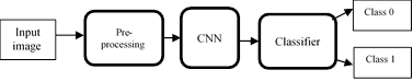
Figure 1. Block diagram of the proposed method
Dataset (input)
The Kaggle website provides a collection of high-resolution images with different imaging conditions. A physician (pathologist) has ranked the data according to the severity of DR in each image. The dataset that has been used in this article contains 35000 eye fundus images of diabetics and healthy people, which can be used in the process of training and testing.
Pre-processing
Data preparation step is the most important and time consuming stage of the implementation of the problem. Since the data are considered as inputs of the project, the higher accuracy of this input leads to a more accurate output; and the garbage in, garbage out incident can be avoided. Before using the images in the process of training and testing, it is necessary to do some pre-processing to ensure that the dataset is consistent and only displays the relevant features. In other words, for creating clarity and brightness in one part of the picture, the periphery can be faded and darkened. In this procedure, the background is intentionally rendered blurry so the main parts of the image can be viewed clearly. Using the Gaussian blur and weighted addition of the original image with the processed image, the irrelevant parts of the background flatten out and some parts of the image that correspond to the blood vessels and nodes in the retina stand out. So, fewer operations are needed for feature extraction. Also, normalization function is applied to the image to cover the image area with fixed dimensions. The purpose of normalization is to eliminate image defects. After the image pre-processing operation, images with the size 512×512 are fed to the CNN.
Proposed architecture
CNN is very similar to artificial neural network. The network input consists of neurons with trainable weights and biases. Each neuron receives a number of inputs and then calculates the multiplication of weights in inputs and finally, using an error function which is a nonlinear conversion, generates the result [11].
Since 20، new architectures have been introduced that reduce errors and increase the accuracy in this area. In the year 2015, a number of researchers in Microsoft came up with the ResNet architecture and this architecture reduced the error to 3.6%. This architecture is composed of 152 layers that broke all records in all three categories of object recognition, classification and localization using a model. In fact, this model is trained to use the human object recognition power and detects the objects far better than humans. There are different versions of this architecture, e.g. with 22 layers, 34 layers, 52 layers and 152 layers that are used according to the requirements [12].
Table 1, below shows the architectures provided up to the year 2015 with highlighting the advantages of each layer compared to the previous architectures.
Table 1. Introduction of the CNN architectures
|
Method |
Year |
Ranking |
Architecture |
Accomplishment |
|
AlexNet |
2012 |
1st |
5 convulsion layers + 3 fully connected layers |
Important architecture that attracted many researchers to computer vision area |
|
ZF Net |
2013 |
1st |
5 convulsion layers + 3 fully connected layers |
Reduced errors and increased efficiency |
|
Clarifai |
2013 |
1st |
5 convulsion layers + 3 fully connected layers |
Showing the events that occurs within the network |
|
VGG |
2014 |
2nd |
13-15 convulsion layers + 3 fully connected layers |
Complete assessment of the network with incremental depth |
|
GoogLeNet |
2014 |
1st |
21 convulsion layers + 1 fully connected layers |
Increasing the depth and width of the network without the need to increase computing |
|
ResNet
|
2015 |
1st |
152 convulsion layers + 1 fully connected layers |
Increasing the depth of the network and providing the means to prevent gradient saturation and reducing error |
For the implementation of this model, according to the size of the dataset and the complexity of the problem, the ResNet34 architecture is used which has 34 blocks. These blocks contain Convulsion Layer, Max Pooling Layer and Average Pooling Layer. The input layer contains raw image pixel values, an image with a height of 512 and width of 512 and 3 colour channels of blue, red, and green (512×512×3). This model has optimum weights that are stored on the ImageNet database and it is one of the most popular CNN network architectures for training. In this problem, the data can be divided into two groups. The first group contains healthy images and their number in the training problem is 25 thousand images, and the second group relates to the images that do not show diabetes and their number in training problem is 9 thousand images. The problem consists of two classes: 0 and 1 (healthy and with diabetes). In the implementation of this architecture, 22 Convulsion Layers, 1 Max Pooling Layer, and 1 Average Pooling Layer were used. The conv1 layer uses a 7×7 filter and 2 strides and 3 paddings; the conv2 layer uses a 3×3 filter and 1 stride and 1 padding; and Max Pooling layer uses a 3×3 filter and 2 strides and 2 paddings. The reason for the use of Max Pooling is its faster convergence, better generalization (improvement of generalization) and choosing more invariable features.
In recent years, there have been several types of quick implementation of CNN networks on the GPU which mostly use the Max pooling operation. Also, Max Pooling and Average Pooling are very useful for deformation management. Also, the RELU activation function was used in the form of a layer that applies the activation function to every single element. The most common form of a CNN architecture is a combination of a few RELU-CONV layers and after that, pooling layers are placed and this template is repeated till the input image is reduced to the desired size. Meanwhile, layers such as Average Pooling can be used as well. The last layer contains the output, such as a rating of categories. In this implementation, a few convulsion layers are placed before each Max Pooling layer. Generally, this method is a good idea for large and deep networks because several combined convulsion layers can obtain more sophisticated features from the input mass before they are lost during the pooling operation.
Training phase
Neural network training consists of determining the appropriate weights for the neural network. For this purpose, a powerful and fast optimization method must be used. Since neural network training for small datasets can result in over-fitting, the purpose of the convulsion layer is extraction of patterns, e.g. finding the sequence of distinctive patterns in the input which usually occur all along the training data.
Test phase
The test phase comes after the training phase, and the model accuracy in label prediction can be evaluated. In the test phase a new image is fed to the network and all the things that were done in the training phase are also repeated in this phase. The only difference of this step with the training step is the lack of error back propagation phase. Here, merely the input is multiplied by weight values that were set at the training stage and finally, after doing all the calculations, a number appears at the end of the network.
Hardware and software used in operations
The CNN network runs on a GPU using two NVIDIA Geforce GTX 1080 graphic cards and an Intel Core-i7 CPU. For the implementation, the Python OpenCV programming language is used based on Pytorch platform, which is one of the powerful platforms in the field of machine learning, and it is also supported by Facebook Co.
Implementation result
In this problem, the data were divided into two classes. The first class is related to the images of diabetic patients that includes 25 thousand images, and the second class is related to the images of people that do not have diabetes that includes 9 thousand images. In the test phase, about 2000 images of healthy and diabetic people were used. The training and testing time for this problem was 180 seconds, the greater part of which was used for training and the rest for testing the model. After completing the runtime of the program source code, the result was obtained.
Results and discussion
In pre-processing step, the Gaussian filter and weighted addition is used. Filtering is one of the basic operations often referred to as a pre-processing in signal processing (Figure 2a and 2 b). It has a variety of applications in image enhancement, noise elimination and edge detection. The Gaussian filter is a low-pass filter and deletes high frequencies of the image and produces an image with low frequencies. The effect of applying this filter on the image is a smooth or blurry image.


(a) Original image (b) Image after pre-processing
Figure 2. Image pre-processing phase
The higher the value of central weight, the more image detail is preserved but the noise will not be removed completely. On the contrary, if the central weight is low, more noise will be eliminated but the image details, including the edges of the image, will be lost. To improve the image quality and detection of the central part of the image, a weight of 4 for the original image and a weight of 10 for the filtered image was considered. It can be seen that in the filtered image, lesions and blood vessels are visible and extraction of micro aneurysms and other features are done with greater speed and accuracy (Figure 3).
![]()
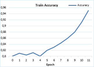
Figure 3. Diagram of accuracy in training phase, on the basis of the number of repetitions or Epoch
Accuracy in training phase
In the training phase of this problem, the data have been divided into two groups. The first group contains data relating to people with the diabetes and its number for the training problem was 25 thousand images, and the second group relates to the images of the people who do not have diabetes and its number for the training problem was about 9 thousand images. In this way, the problem is split into separate sub-problems and at any time, one of the sub-problems (with keeping constant the decision variables available in other sub-problems) is optimized with the best known value; then another sub-problem is considered and this action will repeat until the satisfactory answer is reached. Across various layers, different mappings of and input data will be obtained and at the same time, usually dimension reduction happens as well.
Finally, the network has the data that are fed to different neurons and their weights are adjusted accordingly. After these weights were adjusted properly, the training phase is over. At this stage, the number of repetitions or Epoch has been 11 times and as shown in the diagram, the accuracy up to Epoch 4 shows an ascending and descending curve, but from the 5th Epoch onward, due to choosing more efficient weights than before, the accuracy has increased dramatically and in Epoch 11 accuracy is equal to 95% (Figure 4).
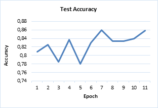
Figure 4. Diagram of accuracy in test phase, on the basis of the number of repetitions or Epoch
Accuracy in test phase
After the training phase, the testing phase begins. In this problem, the number of test images is approximately 2000 diabetic and healthy images with class 0 and class 1 labels. At the end of the network, some neurons are determined to represent each class and their weights are automatically set so that every time a particular class is to be imported, the relevant neuron gives the highest output. After detecting the type of class, the pictures are placed in one of the classes 0 or 1 (normal or diabetic). According to the graph in Figure 4, the accuracy of both classes from the Epoch 0 to Epoch 5 has been alternately ascending and descending, and it reflects a bad choice of weights but from the Epoch 6, accuracy has increased dramatically and in Epoch 11 it is equal to 86%. In CNN, the main objective is reducing the amount of loss through weight modification and this weight modification is done via the Adam optimization function which is a gradient-based optimization algorithm. The goal of optimization is to determine the design variables, such that the target function becomes minimum or maximum.
Table 2. Results obtained from the proposed model
|
Support |
F1-Score |
Recall |
Precision |
Label |
|
1290 |
0.91 |
0.94 |
0.88 |
Class 0 |
|
460 |
0.70 |
0.64 |
0.78 |
Class 1 |
|
1750 |
0.85 |
0.86 |
0.85 |
Avg./total |
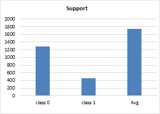
Figure 5. Diagram of the images detected correctly in each class
The Table 2 shows the values for Precision of the system accuracy amongst the predicted data and Recall of the ratio between the number of predicted data to the total expected data for prediction in the test phase, and the averages of each one for classes 0 and 1 has been obtained. According to the obtained values, the Precision and Recall for class 0 had a better result than class 1 and the averages for both classes were 85% Precision and 86% Recall (Figure 5).
Assessment of the proposed model
The F1 criterion is used for evaluation of the system performance. It is a kind of average between the Precision parameter and Recall parameter. In accordance with the following formula, its value is obtainable using the values of Precision and Recall, Eq. (1).
![]() (1)
(1)
Due to the high values of Recall and Precision of the class 0, the F1 value for this class is equal to 91% and for the class 1, it is equal to 70%. The average of the two classes is equal to 85%. The Support column in table 2 shows the number of labels of each class that are detected correctly. It can be seen that from 2000 picture used in the testing phase, 1290 with the label 0 and 460 pictures with the label 1 were detected correctly and the total images that were correctly classified is 1750 images. Approximately, 250 images from 2000 images were not correctly classified and it is likely that the class labels had a problem or those images had no labels at all.
Analysis of the confusion matrix
Figure 6 shows the confusion matrix in which the performance of the proposed algorithm is shown. Each column of the matrix shows an example of the predicted value, while each row shows an example of the real (true) value.
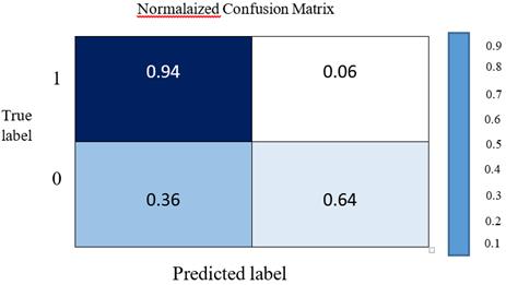
Figure 6. Confusion matrix
This matrix is used to determine the amount of assessment parameters (Precision and Recall). The result of this test is a binary classification (two classes) and the data are split into two positive and negative groups.
The values available in any part of the matrix are obtainable as follows:
Row 0 Column 0 = True Positive, the ill person is correctly diagnosed as ill and its value is 94%.
Row 0 Column 1 = False Positive, the healthy person is incorrectly diagnosed as ill and its value is 6%.
Row 1 Column 0 = False Negative, the ill person is incorrectly diagnosed as healthy and its value is 36%.
Row 1 Column 1 = True Negative, the healthy person is correctly diagnosed as healthy and its value is 64%.
Comparison of the proposed method with Pratt method
In order to provide the results and a more tangible comparison, articles that could achieve the highest accuracy with the use of the above-mentioned architectures are used here. In this section, the proposed method is compared with the method proposed by Pratt. It is noteworthy that the test image collection in Pratt’s research contained 5000 images categorized in 5 classes. Because the number of classes in the proposed method is not equal to the Pratt method, in this section, just the number of images related to the classes 0 and 1 that have been diagnosed properly are compared, and the results are shown in the image detection column in the following Table 3.
Table 3. Comparison of the proposed method with Pratt method
|
Method |
Accuracy |
Sensitivity |
Image detection |
|
Pratt et al 5000 test images |
75% |
95% |
Class 0=3456 images Class 1=179 images |
|
Proposed method 2000 test images |
86% |
85% |
Class 0=1290 images Class 1=460 images |
After comparison of the proposed method with Pratt method, it can be observed that while the number of test images in the proposed method were less than Pratt method, but in the proposed method the number of detected images of class 1 were more than the number of detected images of class1 in Pratt method. So, the accuracy of the proposed method is more than the Pratt method. Also, the sensitivity of the Pratt method is more than the proposed method which is perhaps due to different number of test images and the number of the classes in the problem and this value is more than the value of the sensitivity of the proposed method.
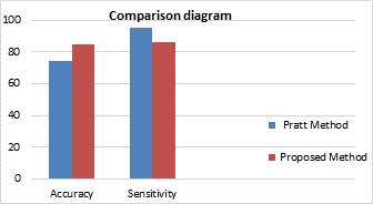
Figure 7. Diagram of comparison of the proposed method with Pratt method
Conclusion
In this article, instead of designing and creation of features manually which is customary in shallow-learning method, a deep conversional network was used that automatically extracts the features available in the image and uses such features to distinguish between images and to identify objects. Here, the important point is that after the learning process, the test would be performed very quickly and easily. In other words, the feature engineering stage in the past methods is replaced with architecture engineering in CNN and other architectures of the deep learning discipline. Also, in the design of the proposed method, the ResNet34 architecture based on CNN was used that offers a better performance than other architectures and could correctly detect a higher number of images than the Pratt method. At present, two-dimensional pictures were used for implementation, but hopefully in the near future, it is possible to improve the detecting capability of this disease through sophisticated three-dimensional images and also in the future by using larger datasets and architectures with more number of layers, the images can be classified in 5 classes.
Acknowledgment
The author wishes to thank the professors of the Faculty of New Medical Technologies at Isfahan University of Medical Sciences, Mr. Dr. Hossein Rabbani, who greatly helped in the choice of the subject and put the necessary datasets and guidelines at his disposal; and also the director of Computer Games Center, Mr. Dr. Javad Rasti, for submitting the computer system to investigate the problem.
References
1. Solanki M.S., Diabetic retinopathy detection using eye images, Artificial Intelligence, Artificial Intelligence Course Project, 2015, p.1-10.
2. Agurto C., Barriga E.S., Murray V., Nemeth S., Crammer R., Automatic detection of diabetic retinopathy and age-related macular degeneration in digital fundus images, Investigative ophthalmology & visual science, 2011, 52, p. 5862-5871.
3. Lazar I., Hajdu A., and Quareshi R.J., Retinal microaneurysm detection based on intensity profile analysis, In 8th International Conference on Applied Informatics, 2010, 1, p. 157–165.
4. Deng L., Yu D., Deep learning: Methods and applications, Foundations and Trends® in Signal Processing, 2014, 7 (3), p. 197-387.
5. Walter T., Massin P., Erginay A., Ordonez R., Jeulin C., and Klein J.C., Automatic detection of micro aneurysms in colour fundus images, Medical image analysis, 2007, 11 (6), p. 555-566.
6. Setiawan W., Damayanti, F., Fundus image classification using two dimensional linear discriminant analysis and support vector machine, International Journal of Advanced Engineering, Management and Science, 2016, 2 (10), p. 1-6.
7. Pratt H., Coenen F., Broadbent D.M., Harding S.P., and Zheng Y., Convolutional neural networks for diabetic retinopathy, Procedia Computer Science, 2016, 90, p. 200-205.
8. Chandore V., Asati Sh., Automatic detection of diabetic retinopathy using deep convolutional neural network, International Journal of Advance Research, Ideas and Innovations in Technology Edition, 2017, 3, p. 633-641.
9. Russakovsky O., Deng J., Su H., Krause J., Satheesh S., Ma S., Fei-Fei L., ImageNet Large scale visual recognition challenge, International Journal of Computer Vision, 2015, 3, p. 211-252.
10. Bengio Y., Learning deep architectures for AI, Foundations and Trends® in Machine Learning, 2009, 2, p. 1-127.
11. He K., Ren S., Sun J., and Zhang X., Deep residual learning for image recognition, IEEE Conference on Computer Vision and Pattern Recognition (CVPR), 2016, p. 770-778.
12. Szegedy Ch., Ioffe S., Vanhoucke V., Alemi A., Inception-v4, Inception-ResNet and the impact of residual connections on learning, Proceedings of the Thirty-First AAAI Conference on Artificial Intelligence (AAAI-17), 2017, 2, p. 4278-4284.