Engineering, Environment
Simulation analysis of natural gas transmission lines using Promax
Nnamdi Emmanuel EZENDIOKWERE *, Victor Joseph AIMIKHE and Boma KINOGOMA
Petroleum and Gas Engineering Department, University of Port Harcourt, Port Harcourt, Nigeria
Email(s): ezendiokwerennamdi@gmail.com, victor.aimikhe@uniport.edu.ng, boma.kinigoma@uniport.edu.ng
*Corresponding author, phone: +2347032747175
Received: April 26, 2018 / Accepted: December 25, 2018 / Published: December 30, 2018
Abstract
In this study, natural gas transmission lines were simulated using Bryan Research and Engineering (BRE) ProMax 2.0 chemical process simulating software. A natural gas composition of methane composition of 90%, was modelled, for which, pipeline length, throughput, suction pressure, line diameter and line temperature were varied. Pipeline lengths of 50,100, 200 miles, throughputs of 200, 250, and 300 MMscfd, suction pressures from 500-10000 psia, line diameters of 20 and 30 inches and gas temperatures of 68- 104⁰F were used. After the simulations, special emphasis was laid on the relationship between total compressor power requirements and pipeline parameters like pipeline pressure drop, length, throughput, and compression station suction pressure in order to evaluate their effects on total compressor horsepower. From more than 1000 data points recorded, it was deduced that there exists, generally, positive correlation between total compressor power and the other pipeline parameters considered. Also, there was a critical pressure drop for each combination of throughput, length and line diameter of a pipeline below which total compressor power significantly varies with pressure drop and above which total compressor power does not change considerably.
Keywords
Pipelines; Compressors; Pressure drop; Promax; Throughput
Introduction
The reliable transportation of processed natural gas from producing areas to where they are needed involves the use of a specialized system of transportation. This is because the natural gas that consumers receive, sometimes, travel long distances before getting to customers. Basically, the transportation system for natural gas consists of specialized network of interconnected pipes, dedicated to bringing natural gas to the doorsteps of gas users [1].
Pipelines in gas transport systems can be grouped into three: gathering, transmission and distribution systems. The gathering lines consists of low pressure, small diameter pipes that carry unprocessed natural gas from well heads to gas processing plants. After processing the gas, natural gas then goes to the transmission system. In gas transmissions lines, gas is carried in high pressure larger diameter pipes over long distances to where the customers reside. While distribution systems consist of another set of low-pressure, small-diameter pipelines whose task is to ultimately take gas to end users like households, factories and power plants [1].
Natural gas transportation requires a lot of energy, usually in the form of pressure energy. And a lot of this energy is spent running compressors in compression stations. Normally, the operating cost of running the compressor stations represents between 25% and 50% of a pipeline company’s operating budget [2].
Therefore, the purpose of this study is to undertake a simulation analysis of gas transmission lines, particularly their total compressor power requirements. This is because the ability to fully understand pipeline parameters and their effects on the total compressor power requirements of gas transmission lines will help in reducing compressor power burdens of natural gas transmission lines. Ultimately, research outcomes developed here will become useful insights, especially, in the hands of pipeline design engineers.
Material and method
A simplified working algorithm used for the simulations done in this study using a flow chart (Figure 1). The following procedure was used for the ProMax simulations:
(a) Open the ProMax simulation software by either double clicking on BRE ProMax shortcut on desktop or the ProMax icon initially pinned to taskbar.
(b) The ProMax software will open revealing a small dialogue window at the center of the screen.
(c) Click on the blank project radio button to start a new project, causing a blank flow sheet to open simultaneously opening a shapes window on the left side of the screen.
(d) Since a gas transmission line is being simulated, click and drag the following blocks from the shapes window to the center of the blank flowsheet.
· a compressor from fluid drivers group of blocks.
· a heat exchanger (after cooler) from heat exchangers.
· a pipe section from miscellaneous.
· a two-phase vertical separator from separators.
(e) In the case of 100 and 200 miles pipeline sections, also click and drag a cross flowsheet connector to flowsheet. The blocks will turn red until they are properly connected.
(f) Assign an environment to the flowsheet by clicking on the environment icon in ProMax menu, choose the Soave Redlich Kwong (SRK) property package and install the following components: Nitrogen, carbon (iv) oxide, methane, ethane, propane, iso-butane, butane, iso-pentane, pentane, and hexane.
(g) Click on the pointer icon in ProMax tools bar to change the cursor to connector mode.
(h) Connect the process streams first by connecting appropriate process stream connection point on each block.
(i) Next click on the energy streams icon at the bottom of the shapes window to change the cursor to energy stream connection mode.
(j) Connect the appropriate energy streams from the compressor to the gas pipeline.
(k) If the connections are right, the blocks will change from red to blue.
(l) Double click on each on each stream and block to set the relevant specifications. The streams and blocks will all turn green if the right number of correct specifications are made.
(m) Run the simulation by clicking on the solve button with a capital letter p on top of an inverted chevron character in the project viewer window.
(n) Warnings displayed in different colors in a small window under the flowsheet in the main window should serve as hints in cases of unsuccessful simulations.
(o) To generate a report at the end of a successful simulation, click on the report icon on the ProMax menu in the main window, and choose items to include in the report after indicating the report file format.
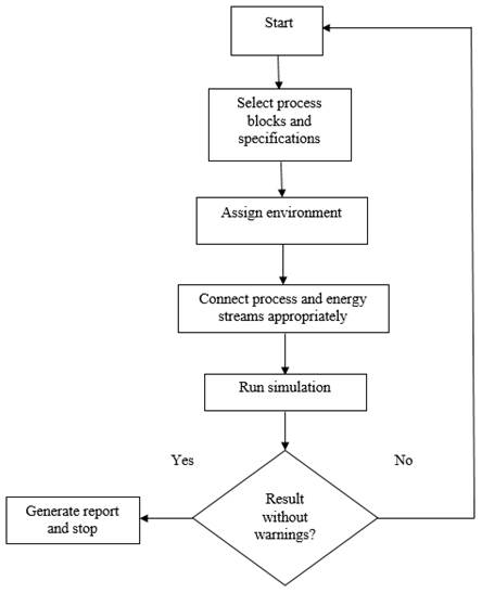
Figure 1. ProMax simulation flow chart
Figure 2 shows a schematic diagram of a simple 50-mile gas transmission line model used for the simulation.
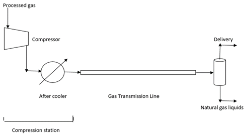
Figure 2. Schematic diagram of a simple gas transmission line model
The procedure represented above was used to simulate 50-mile, 100-mile and 200-mile long natural gas transmission lines. Using the different combinations of pipeline length, pipeline diameter, gas flow rate, and compositions, over a thousand simulations were done. In other to ensure that the simulated gas transmission lines were as close to their real life counterparts as possible, the whole length of the lines was divided into 50 mile sections by compression stations, with each section containing at least three (3) valve stations. The valve stations were positioned after every 20 miles, except when the valve station occurs very close to a compression station.
Table 1 shows the natural gas composition used for the simulation.
Table 1. Composition of natural gas used for simulation
|
Composition |
Mole percent (%) |
|
C1 |
90.0 |
|
C2 |
4.20 |
|
C3 |
2.68 |
|
i-C4 |
1.08 |
|
n-C4 |
0.17 |
|
i-C5 |
0.02 |
|
n-C5 |
0.01 |
|
n-C6 |
0.02 |
|
CO2 |
0.55 |
|
N2 |
1.27 |
A processed sweet natural gas with composition similar to TransCanada transmission line gas was used. The processed sweet natural gas has a methane composition of 90%. But, the sweet gas composition had carbon (iv) oxide and nitrogen compositions of 0.55 and 1.27 mole percent respectively.
Also, to maintain accuracy of the simulation, different flow sheets were used for each 50-mile gas transmission line section. The different flow sheets were then joined using Promax cross-flow sheet connector to ensure proper exchange of both process and energy streams between flow sheets. For the choice of equation of state, the Soave Redlich Kwong (SRK) equation of state was used. Although, Peng Robinson could have been used, but SRK gives better results when compared with Peng Robinson for natural gas applications.
Begs and Brill multiphase correlation was used because of its wide acceptance in the oil and gas industry. For the pipe, a buried standard steel pipe of overall heat transfer coefficient of 0.25 W/m2-oK was used. This allows some heat to escape through the pipe wall into the surrounding. An after cooler was also added after each compressor to ensure that the temperature of the sweet gas after compression does not exceed 1000F. A polytropic efficiency of 80% and a compression ratio of 2 was chosen to avoid unnecessarily overheating of the gas in transit. This was done because compressor stations at gas transmission lines normally have compression ratios of 2 [3].
Considering the effect of flow rate on gas transportation in general, three (3) different flow rates were considered while simulating the gas transmission lines, they include: 200,250, and 300 MMSCFD. Due to the fact that Promax gives accurate results only for pipeline simulations with pressure drop less than 10%, any simulation result with pressure drop above 10% of the pipeline inlet pressure in any pipe section was discarded. This was done to preserve the integrity of the generated Promax data. Steps between data points were deliberately made small in other to preserve accuracy.
Results and discussion
Figure 3 shows an example of the graphical plot of compressor power requirement against total line pressure drop for different combinations of transmission pipeline length, line diameter, and gas flow rate. Plots for other pipe lengths were predominantly of this shape.
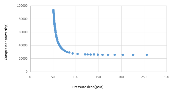
Figure 3. Graph of compressor power requirements against pressure drop for 100 mi, 20”, 200MMSCFD, 68⁰F
From the graphs by Figure 3, generally, as total line pressure drop increases, total compressor requirements decreases. But, a closer look at the graphs as represented by Figure 3 will reveal three prominent behaviors between compressor requirement and the accompanying pressure loss. For the first part of the plot (low pressure drop range), corresponding to very high line pressures, small changes in total line pressure drop lead to significantly large changes in compressor power.
After that almost linear relationship, each curve then experiences a change in direction, before finally levelling out. For this last part of each curve, corresponding to lower pipeline pressures, the compressor power does not significantly change, even as total line pressure drop increases. This behavior can be attributed to the fact that at higher pipeline pressures, slight changes in conditions normally create big pressure waves that are easily transmitted throughout the whole pipeline system. But, changes at low pressures are hardly felt, since pipeline transportation is primarily facilitated by changes in pressure energy.
Table 2. Summary of results from ProMax simulations
|
Pipeline Length (mi) |
Gas flow rate (MMscfd) |
Pipeline Diameter (in) |
Critical pressure drop (psia) |
Compressor Power (hp) |
|
50 |
200 |
20 |
55.3552 |
8235.77 |
|
30 |
6.39278 |
8235.77 |
||
|
250 |
20 |
86.9493 |
9183.53 |
|
|
30 |
9.97234 |
9183.53 |
||
|
300 |
20 |
107.282 |
12434.2 |
|
30 |
12.3460 |
12434.2 |
||
|
100 |
200 |
20 |
103.5659 |
26962.96 |
|
30 |
11.97024 |
26847.32 |
||
|
250 |
20 |
170.3547 |
32813.45 |
|
|
30 |
21.46403 |
32845.85 |
||
|
300 |
20 |
278.5072 |
39301.3 |
|
|
30 |
30.91819 |
39600.8 |
||
|
200 |
200 |
20 |
205.9134 |
36206.43 |
|
30 |
22.75965 |
37276.36 |
||
|
250 |
20 |
313.6289 |
45767.02 |
|
|
30 |
35.23813 |
46773.51 |
From the aforementioned simulations, a summary of the relationship among various parameters was obtained, as captured in Table 2 above. Specifically, total compressor power increases as the pipeline length increases, as can be seen from Table 2.
Also, in Table 2, it can be deduced that the total compressor power increases as throughput increases. Hence, from the table, it can be deduced that the relationship between total compressor power requirement and the pipeline parameters considered can be generally described as positive correlation.
Especially, there was positive correlation between total compressor power and critical pressure drop. Where the critical pressure drop is taken as the total line pressure drop value corresponding to the point on the total compressor power-total pressure drop graph at which the curve begins to flatten out. And this general trend between total compressor requirements and other pipeline parameters is basically true. This is because, increased flow rate means more gas is being transported, and the larger the quantity of gas, the longer the lines, the bigger the diameter and the bigger the compression power that will naturally be needed. Ultimately, leading to higher pressure drop due friction in the pipelines.
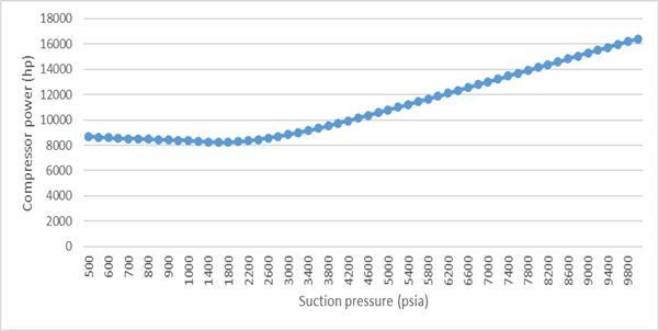
Figure 4. A plot showing the relationship between compressor power and suction pressure
The relationship between suction pressures and compressor power was shown graphically in Figure 4 above. While, for suction pressures, the compressor power generally, increases as line pressure increases. But, a closer look will reveal that there was an initial dip or decrease in compressor power requirement as suction pressure increased. And then, continuous increase in compressor power as suction pressure increased. The dip in the curve can be attributed to the effect of the value of compressibility factor (z). This is because, as pressure increases, z-factor first decreases in value until it reaches a minimum, before it starts increasing as the pressure increases [3].
Conclusion
From the study, the following conclusions can be drawn:
(a) Gas transmission line total compressor power requirement increases as the transmission line length increases.
(b) Gas transmission line total compressor power requirement increases as the transmission line throughput increases.
(c) Gas transmission line total compressor power requirement increases as the transmission compressor station suction pressures increases.
(d) There was a critical pressure drop for each combination of throughput, length and line diameter of a pipeline below which compressor power significantly varies with pressure drop and above which compressor power does not change considerably.
References
1. Rios M. and Borraz S., Optimization problems in natural gas transportation systems: A state-of-the-art review, Applied Energy, 147, p. 536-555.
2. Luongo C.A., Gilmour B.J., and Schroeder D.W., Optimization in natural gas transmission networks: A tool to improve operational efficiency, Technical report, Stoner Associates, Inc., Houston, 1989.
3. Chi U.I, Natural gas production engineering, John Wiley & Sons, Inc., 1992.
4. Agwu O.E., Markson I.E., Umana M.O., Minimizing energy consumption in compression stations along two gas pipelines in Nigeria, American Journal of Mechanical Engineering and Automation, 2016, 3 (4), p. 29-34.
5. Agwu O., Eleghasim C., Mechanical drive gas turbine selection for service in two natural gas pipelines in Nigeria, Case Studies in Thermal Engineering, 2017, 10, p. 19-27.
6. Aimikhe V., Kinigoma B. and Iyagba E., Predicting the produced boil off gas in the moss spherical liquefied natural gas (LNG) Vessel, SPE Nigeria Annual International Conference and Exhibition, 2013.
7. Amyx J.W., Bass D.M. Jr., and Whiting R.L., Petroleum reservoir engineering-physical properties, New York: McGraw-Hill, 1960.
8. Armstrong J.S., Illusions in regression analysis, International Journal of Forecasting, 2012, 28 (3), 689.
9. Campbell J.M., Gas conditioning and processing, Norman, Oklahoma, Campbell Petroleum Series, 1976.
10. Comodi G., Renzi M., Caresana F., Pelagalli L., Enhancing micro gas turbine performance in hot climates through inlet air cooling vapor compression technique, Appl. Energy, 2015, 147, p. 40-48.
11. David A.F., Statistical models: Theory and practice, Cambridge University Press, 2005.
12. McCain W.D., Jr., The properties of petroleum fluids, Tulsa: Petroleum Publishing, 1973.
13. Mohammad M.G. and Alireza B., A new correlation for accurate estimation of natural gases water content, Journal of Petroleum and coal, 2014.
14. Moshfeghian M., Dense transportation of natural gas, Campbell January Tip of the Month, 2010.
15. Musaab M.A. and Mohammed A.A., A comprehensive study on the current pressure drop calculation in multiphase vertical wells, Current Trends and Future Perspectives, Journal of Applied Sciences, 2014, 14, p. 3162-3171.
16. Sa A.D., Al Zubaidy S., Gas turbine performance at varying ambient temperatures, Appl. Thermo Eng., 2011, 31, p. 2735-2739.
Appendix
Table A1. Promax results for a 100 mi, 20 and 30 in pipelines with gas flowrate of 200 MMScfd
|
100mi |
20" |
200MMSCFD |
68⁰F |
|||||
|
P(Feed)(psia) |
Comp1(hp) |
Comp2(hp) |
P2(Psia) |
T2 (˚F) |
∆P1(Psia) |
∆P2(psia) |
∑∆P(psia) |
∑Comp(hp) |
|
500 |
8004.85 |
17535.4 |
3117.53 |
73.3753 |
200.456 |
55.6459 |
256.1019 |
25540.25 |
|
550 |
7953.78 |
17567.3 |
3621.18 |
73.4149 |
175.927 |
50.1091 |
226.0361 |
25521.08 |
|
600 |
7904.42 |
17620.3 |
4101.08 |
73.3388 |
156.888 |
46.3658 |
203.2538 |
25524.72 |
|
650 |
7856.82 |
17692 |
4564.81 |
73.2231 |
141.638 |
43.6416 |
185.2796 |
25548.82 |
|
700 |
7811.12 |
17781.2 |
5016.88 |
73.0983 |
129.142 |
41.5539 |
170.6959 |
25592.32 |
|
750 |
7767.21 |
17886.8 |
5460.19 |
72.8607 |
118.728 |
39.8927 |
158.6207 |
25654.01 |
|
800 |
7725.2 |
18008.5 |
5896.74 |
72.7537 |
109.933 |
38.5323 |
148.4653 |
25733.7 |
|
850 |
7685.13 |
18245.7 |
6327.91 |
72.6552 |
102.424 |
37.393 |
139.817 |
25930.83 |
|
900 |
7647.06 |
18298.2 |
6754.75 |
72.5646 |
95.9566 |
36.4218 |
132.3784 |
25945.26 |
|
950 |
7611.03 |
18465.3 |
7178.04 |
72.4814 |
90.3442 |
35.5815 |
125.9257 |
26076.33 |
|
1000 |
7577.08 |
18646.6 |
7598.39 |
72.2081 |
85.442 |
34.8457 |
120.2877 |
26223.68 |
|
1200 |
7463.02 |
19499.9 |
9258.59 |
72.0046 |
70.9477 |
32.6182 |
103.5659 |
26962.92 |
|
1400 |
7385.67 |
20250.2 |
10897.2 |
71.8475 |
61.6704 |
31.0965 |
92.7669 |
27635.87 |
|
1600 |
7346.83 |
21658.6 |
12533.6 |
71.7224 |
55.3552 |
29.9786 |
85.3338 |
29005.43 |
|
1800 |
7347.13 |
22576.5 |
14142.6 |
71.6203 |
50.8287 |
29.1168 |
79.9455 |
29923.63 |
|
2000 |
7385 |
24146.8 |
15756.8 |
71.5355 |
47.4415 |
28.429 |
75.8705 |
31531.8 |
|
2200 |
7457.25 |
25451.1 |
17367.9 |
71.4637 |
44.8153 |
27.8658 |
72.6811 |
32908.35 |
|
2400 |
7559.34 |
26777.3 |
18976.7 |
71.4022 |
42.77189 |
27.3952 |
70.16709 |
34336.64 |
|
2600 |
7687.13 |
28227.9 |
20584 |
71.3489 |
41.0048 |
26.9956 |
68.0004 |
35915.03 |
|
2800 |
7835.52 |
29467.4 |
22190 |
71.3023 |
39.5752 |
26.6515 |
66.2267 |
37302.92 |
|
3000 |
8000.71 |
30822.2 |
23795.2 |
71.2611 |
38.363 |
26.3522 |
64.7152 |
38822.91 |
|
3200 |
8179.34 |
32179.9 |
25399.6 |
71.2244 |
37.3207 |
26.0891 |
63.4098 |
40359.24 |
|
3400 |
8368.68 |
33579 |
27003.5 |
71.1916 |
36.4137 |
25.856 |
62.2697 |
41947.68 |
|
3600 |
8566.66 |
34898.1 |
28606.9 |
71.1621 |
35.6163 |
25.6479 |
61.2642 |
43464.76 |
|
3800 |
8771.37 |
36256.5 |
30209.9 |
71.1353 |
34.9092 |
25.461 |
60.3702 |
45027.87 |
|
4000 |
8981.52 |
36613.7 |
31812.6 |
71.111 |
34.2771 |
25.2922 |
59.5693 |
45595.22 |
|
4200 |
9196 |
38969.2 |
33415 |
71.0887 |
33.7083 |
25.1389 |
58.8472 |
48165.2 |
|
4400 |
9413.97 |
40322.9 |
35017.2 |
71.0683 |
33.1934 |
24.9991 |
58.1925 |
49736.87 |
|
4600 |
9634.71 |
41674.6 |
36619.2 |
71.0495 |
32.7246 |
24.8711 |
57.5957 |
51309.31 |
|
4800 |
9857.69 |
43024.3 |
38221.1 |
71.0321 |
32.296 |
24.7534 |
57.0494 |
52881.99 |
|
5000 |
10082.5 |
44371.4 |
39822.7 |
71.016 |
31.9022 |
24.6448 |
56.547 |
54453.9 |
|
5200 |
10308.6 |
45716.5 |
41424.3 |
71.0011 |
31.5391 |
24.4553 |
55.9944 |
56025.1 |
|
5400 |
10536 |
45059.4 |
43025.7 |
71.9871 |
31.203 |
24.451 |
55.654 |
55595.4 |
|
5600 |
10764.2 |
48400.2 |
44627.1 |
70.9871 |
30.891 |
24.3643 |
55.2553 |
59164.4 |
|
5800 |
10993.1 |
49738.8 |
46228.3 |
70.9741 |
30.6 |
24.2833 |
54.8833 |
60731.9 |
|
6000 |
11222.6 |
51075.3 |
47829.5 |
70.9619 |
30.329 |
24.2075 |
54.5365 |
62297.9 |
|
6200 |
11452.4 |
52409.7 |
49430.6 |
70.9505 |
30.0749 |
24.1366 |
54.2115 |
63862.1 |
|
6400 |
11682.6 |
53742.2 |
51031.6 |
70.9398 |
29.8365 |
24.0699 |
53.9064 |
65424.8 |
|
6600 |
11912.9 |
55072.7 |
52632.5 |
70.9297 |
29.6123 |
24.0072 |
53.6195 |
66985.6 |
|
6800 |
12143.4 |
56401.2 |
54233.4 |
70.9201 |
29.4009 |
23.9481 |
53.349 |
68544.6 |
|
7000 |
12373.9 |
57728.1 |
53834.3 |
70.9111 |
29.2014 |
23.8924 |
53.0938 |
70102 |
|
7200 |
12604.5 |
59033.1 |
57435.1 |
70.9026 |
29.0127 |
23.8395 |
52.8522 |
71637.6 |
|
7400 |
12835 |
60376.4 |
59035.9 |
70.8945 |
28.8339 |
23.7895 |
52.6234 |
73211.4 |
|
7600 |
13065.3 |
61698 |
60636.6 |
70.8868 |
28.6642 |
23.7421 |
52.4063 |
74763.3 |
|
7800 |
13295.6 |
63098 |
62237.3 |
70.8795 |
28.5029 |
23.0697 |
51.5726 |
76393.6 |
|
8000 |
13525.8 |
64336.5 |
63958.3 |
65.3139 |
28.3495 |
23.6542 |
52.0037 |
77862.3 |
|
8200 |
13755.9 |
65653.5 |
65558.3 |
65.3087 |
28.2032 |
23.6134 |
51.8166 |
79409.4 |
|
8400 |
13985.8 |
66969 |
67158.4 |
65.3037 |
28.0637 |
23.5745 |
51.6382 |
80954.8 |
|
8600 |
14215.4 |
68283.1 |
68758.5 |
65.2989 |
27.9305 |
23.5374 |
51.4679 |
82498.5 |
|
8800 |
14444.9 |
69595.8 |
70358.5 |
65.2944 |
27.803 |
23.502 |
51.305 |
84040.7 |
|
9000 |
14674.2 |
70907.2 |
71958.5 |
65.29 |
27.6811 |
23.502 |
51.1831 |
85581.4 |
|
9200 |
14903.3 |
72217.4 |
73558.6 |
65.2859 |
27.5642 |
23.4681 |
51.0323 |
87120.7 |
|
9400 |
15132.1 |
73526.3 |
75158.6 |
65.2819 |
27.452 |
23.4045 |
50.8565 |
88658.4 |
|
9600 |
15360.7 |
74834 |
76758.7 |
65.278 |
27.3444 |
23.3747 |
50.7191 |
90194.7 |
|
9800 |
15589.1 |
76140.6 |
78358.7 |
65.27443 |
27.241 |
23.3461 |
50.5871 |
91729.7 |
|
10000 |
15817.2 |
77446 |
79958.8 |
65.2708 |
27.1415 |
23.3186 |
50.4601 |
93263.2 |
|
30" |
||||||||
|
500 |
8004.85 |
17534.9 |
3885.96 |
67.7792 |
20.8581 |
5.61079 |
26.46889 |
25539.75 |
|
550 |
7953.78 |
17559.1 |
4294.9 |
67.626 |
18.7005 |
5.29775 |
23.99825 |
25512.88 |
|
600 |
7904.42 |
17600.7 |
4702.23 |
67.4767 |
16.9299 |
5.05164 |
21.98154 |
25505.12 |
|
650 |
7856.82 |
17660.3 |
5108.32 |
67.3371 |
15.4563 |
4.85279 |
20.30909 |
25517.12 |
|
700 |
7811.12 |
17737.2 |
5513.45 |
67.2091 |
14.2143 |
4.68854 |
18.90284 |
25548.32 |
|
750 |
7767.21 |
17831 |
5917.82 |
67.0928 |
13.1571 |
4.55038 |
17.70748 |
25598.21 |
|
800 |
7725.2 |
17941.8 |
6321.57 |
66.9873 |
12.2497 |
4.43238 |
16.68208 |
25667 |
|
850 |
7685.13 |
18069.2 |
6724.81 |
66.8916 |
11.4653 |
4.33029 |
15.79559 |
25754.33 |
|
900 |
7647.06 |
18212.9 |
7127.63 |
66.8046 |
10.7831 |
4.24099 |
15.02409 |
25859.96 |
|
950 |
7611.03 |
18372.5 |
7530.09 |
66.7254 |
10.1864 |
4.16217 |
14.34857 |
25983.53 |
|
1000 |
7577.08 |
18547.5 |
7932.26 |
66.6531 |
9.66201 |
4.092 |
13.75401 |
26124.58 |
|
1200 |
7463.02 |
19384.3 |
9538.74 |
66.418 |
8.09635 |
3.87389 |
11.97024 |
26847.32 |
|
1400 |
7385.67 |
20398.5 |
11142.9 |
66.2446 |
7.08454 |
3.72101 |
10.80555 |
27784.17 |
|
1600 |
7346.83 |
21535.2 |
12745.8 |
66.1117 |
6.39278 |
3.60733 |
10.00011 |
28882.03 |
|
1800 |
7347.13 |
22753.4 |
14347.9 |
66.0235 |
5.89596 |
3.47568 |
9.37164 |
30100.53 |
|
2000 |
7385 |
24024.5 |
15949.5 |
65.9213 |
5.5239 |
3.44878 |
8.97268 |
31409.5 |
|
2200 |
7457.25 |
25329.9 |
17550.7 |
65.8507 |
5.23541 |
3.39112 |
8.62653 |
32787.15 |
|
2400 |
7559.34 |
26657.2 |
19151.6 |
65.7913 |
5.00522 |
3.34301 |
8.34823 |
34216.54 |
|
2600 |
7687.13 |
27998.6 |
20752.4 |
65.7406 |
4.81716 |
3.30223 |
8.11939 |
35685.73 |
|
2800 |
7835.52 |
29348.8 |
22353.1 |
65.6968 |
4.66049 |
3.26721 |
7.9277 |
37184.32 |
|
3000 |
8000.71 |
30704.1 |
23953.7 |
65.6586 |
4.52781 |
3.23681 |
7.76462 |
38704.81 |
|
3200 |
8179.34 |
32062.3 |
25554.1 |
65.6249 |
4.41388 |
3.21017 |
7.62405 |
40241.64 |
|
3400 |
8368.68 |
33421.6 |
27154.6 |
65.595 |
4.31489 |
3.18662 |
7.50151 |
41790.28 |
|
3600 |
8566.66 |
34781 |
28754.9 |
65.5683 |
4.22799 |
3.16566 |
7.39365 |
43347.66 |
|
3800 |
8771.37 |
36139.6 |
30355.2 |
65.5443 |
4.15106 |
3.14689 |
7.29795 |
44910.97 |
|
4000 |
8981.52 |
37496.9 |
31955.5 |
65.5226 |
4.0824 |
3.12997 |
7.21237 |
46478.42 |
|
4200 |
9196 |
38852.5 |
33555.8 |
65.5029 |
4.02073 |
3.11465 |
7.13538 |
48048.5 |
|
4400 |
9413.97 |
40206.2 |
35156 |
65.4849 |
3.96498 |
3.10071 |
7.06569 |
49620.17 |
|
4600 |
9634.71 |
41557.9 |
36756.3 |
65.4684 |
3.91433 |
3.08798 |
7.00231 |
51192.61 |
|
4800 |
9857.69 |
42907.4 |
38356.5 |
65.4533 |
3.86806 |
3.07631 |
6.94437 |
52765.09 |
|
5000 |
10082.5 |
44254.7 |
39956.8 |
65.4393 |
3.82566 |
3.06556 |
6.89122 |
54337.2 |
|
5200 |
10308.6 |
45599.7 |
41556.8 |
65.4264 |
3.78662 |
3.05564 |
6.84226 |
55908.3 |
|
5400 |
10536 |
46942.6 |
43157 |
65.4144 |
3.75054 |
3.04645 |
6.79699 |
57478.6 |
|
5600 |
10764.2 |
48283.2 |
44757.1 |
65.4032 |
3.7171 |
3.03791 |
6.75501 |
59047.4 |
|
5800 |
10993.1 |
49621.7 |
46357.2 |
65.3927 |
3.68601 |
3.02997 |
6.71598 |
60614.8 |
|
6000 |
11222.6 |
50958 |
47957.3 |
65.383 |
3.65701 |
3.02255 |
6.67956 |
62180.6 |
|
6200 |
11452.4 |
52292.4 |
49557.5 |
65.3738 |
3.62991 |
3.01562 |
6.64553 |
63744.8 |
|
6400 |
11682.6 |
53624.7 |
51157.6 |
65.3653 |
3.60452 |
3.00911 |
6.61363 |
65307.3 |
|
6600 |
11912.9 |
54955.1 |
52757.7 |
65.3572 |
3.58067 |
3.00301 |
6.58368 |
66868 |
|
6800 |
12143.4 |
56284.8 |
54357.9 |
65.3495 |
3.52055 |
2.99726 |
6.51781 |
68428.2 |
|
7000 |
12373.9 |
57611.2 |
55958 |
65.3423 |
3.49635 |
2.99185 |
6.4882 |
69985.1 |
|
7200 |
12604.5 |
58935.8 |
57558.1 |
65.3376 |
3.47321 |
2.98674 |
6.45995 |
71540.3 |
|
7400 |
12835 |
60258.7 |
59158.2 |
65.3313 |
3.45106 |
2.98191 |
6.43297 |
73093.7 |
|
7600 |
13065.3 |
61580 |
60758.3 |
65.3252 |
3.4298 |
2.97733 |
6.40713 |
74645.3 |
|
7800 |
13295.6 |
62899.6 |
62358.2 |
65.3194 |
3.46328 |
2.97299 |
6.43627 |
76195.2 |
|
8000 |
13525.8 |
64218 |
63958.2 |
65.3139 |
3.44712 |
2.96888 |
6.416 |
77743.8 |
|
8200 |
13755.9 |
65534.8 |
65558.3 |
65.3087 |
3.43175 |
2.96496 |
6.39671 |
79290.7 |
|
8400 |
13985.8 |
66850.2 |
67158.4 |
65.3037 |
3.4171 |
2.96123 |
6.37833 |
80836 |
|
8600 |
14215.4 |
68164.2 |
68758.4 |
65.2989 |
3.40313 |
2.95768 |
6.36081 |
82379.6 |
|
8800 |
14444.9 |
69476.8 |
70358.5 |
65.2944 |
3.38979 |
2.95429 |
6.34408 |
83921.7 |
|
9000 |
14674.2 |
70788.1 |
71958.5 |
65.29 |
3.37703 |
2.95105 |
6.32808 |
85462.3 |
|
9200 |
14903.3 |
72098.1 |
73558.6 |
65.2859 |
3.36482 |
2.94795 |
6.31277 |
87001.4 |
|
9400 |
15132.1 |
73406.9 |
75158.6 |
65.2819 |
3.35312 |
2.94499 |
6.29811 |
88539 |
|
9600 |
15360.7 |
74714.5 |
76758.7 |
65.278 |
3.34191 |
2.94216 |
6.28407 |
90075.2 |
|
9800 |
15589.1 |
76020.9 |
78358.7 |
65.2744 |
3.33115 |
2.93944 |
6.27059 |
91610 |
|
10000 |
15817.2 |
77326.2 |
79958.8 |
65.2708 |
3.32081 |
2.93683 |
6.25764 |
93143.4 |
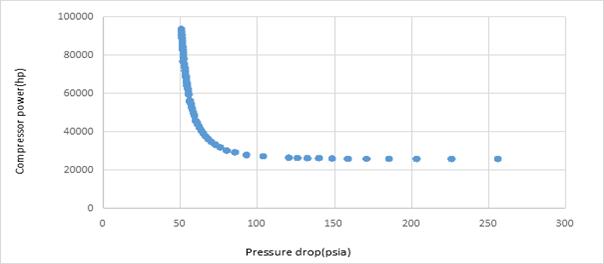
Figure A1. Graph of compressor power requirements against pressure drop for 100 mi, 20”, 200 MMSCFD
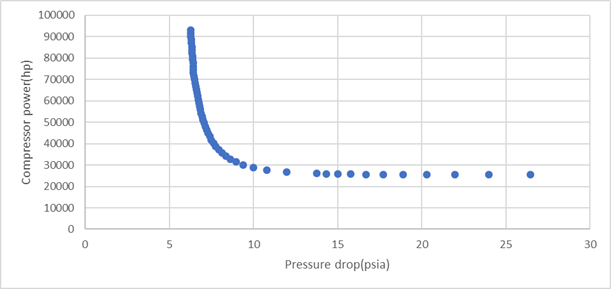
Figure A2. Graph of compressor power requirements against pressure drop for 100mi, 30”, 200 MMSCFD